Wolfram Function Repository
Instant-use add-on functions for the Wolfram Language
Function Repository Resource:
Construct a least-squares trigonometric fit to data
ResourceFunction["TrigFit"][data,n,x] gives the least‐squares trigonometric fit to data up to cos(nx) and sin(nx), with fundamental period 2π. | |
ResourceFunction["TrigFit"][data,n,{x,L}] gives the least‐squares trigonometric fit to data up to cos(2πnx/L) and sin(2πnx/L), with fundamental period L. | |
ResourceFunction["TrigFit"][data,n,{x,x0,x1}] gives the least‐squares trigonometric fit to data up to cos(2πn(x-x0)/(x1-x0)) and sin(2πn(x-x0)/(x1-x0)), with fundamental period x1-x0. |
Generate data corresponding to one period of a periodic function:
| In[1]:= |
Construct a low-order trigonometric fit:
| In[2]:= |
| Out[2]= |
Show the fit along with the original data:
| In[3]:= |
| Out[3]= | 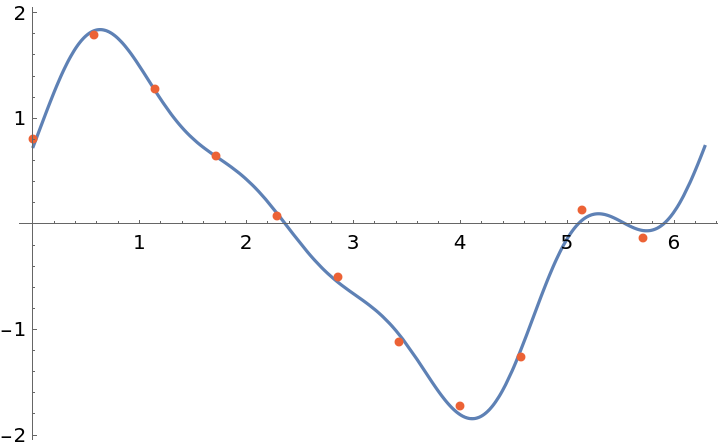 |
Generate samples from a periodic function:
| In[4]:= |
| Out[4]= |
Trigonometric fit over [0,2π]:
| In[5]:= |
| Out[5]= |
Trigonometric fit over [0,ℒ]:
| In[6]:= |
| Out[6]= |
Trigonometric fit over [x0,x1]:
| In[7]:= |
| Out[7]= |
Sample points over a closed curve:
| In[8]:= |
| Out[8]= |  |
Plot the trigonometric fit along with the original data:
| In[9]:= | ![ParametricPlot[
ResourceFunction["TrigFit"][dat, 3, {t, 2 \[Pi]}] // Evaluate, {t, 0,
2 \[Pi]}, Epilog -> {Directive[AbsolutePointSize[4], ColorData[97, 2]], Point[dat]}]](https://www.wolframcloud.com/obj/resourcesystem/images/847/8475605c-8b58-40c7-83ff-46afcfc3ec5f/46ecfd23ed29327c.png) |
| Out[9]= | 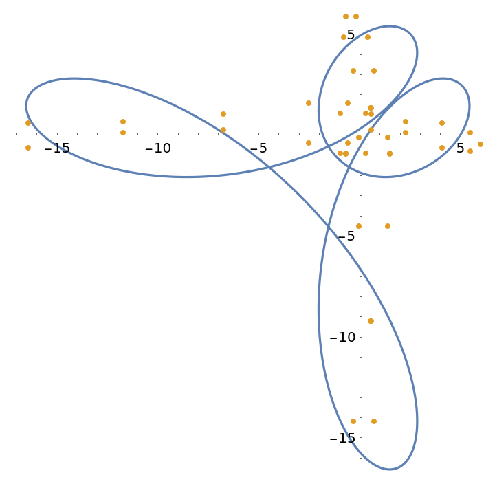 |
Generate samples from a periodic function:
| In[10]:= |
| Out[10]= |
Use TrigFit to construct the trigonometric fit:
| In[11]:= |
| Out[11]= |
Use Fit to construct the trigonometric fit:
| In[12]:= |
| Out[12]= |
Sample points on a knot:
| In[13]:= |
Construct a low-order trigonometric fit from the data:
| In[14]:= |
| Out[14]= |  |
Plot the trigonometric fit of the knot, and compare with the result of KnotData:
| In[15]:= | ![{ParametricPlot3D[f8trig[t], {t, 0, 2 \[Pi]}, Axes -> False, Boxed -> False, Mesh -> None, PlotRange -> All, PlotStyle -> Tube[0.2, Method -> {"Caps" -> False}], ViewPoint -> {0, 0.01, 5}], KnotData["FigureEight"]} // GraphicsRow](https://www.wolframcloud.com/obj/resourcesystem/images/847/8475605c-8b58-40c7-83ff-46afcfc3ec5f/2581737a44ca860c.png) |
| Out[15]= | 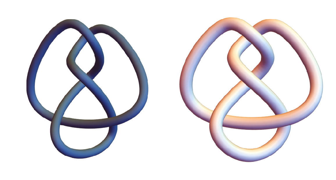 |
This work is licensed under a Creative Commons Attribution 4.0 International License