Function Repository Resource:

FittedModelPlot

Source Notebook

Plot fitted models together with their raw data

Contributed by: Lukas Lang

ResourceFunction["FittedModelPlot"][FittedModel[…]]

plots the raw data and the fit described by the FittedModel[…] expression.

ResourceFunction["FittedModelPlot"][FittedModel[…],lims]

plots the fit over the range given by lims.

ResourceFunction["FittedModelPlot"][{FittedModel[…],FittedModel[…]},…]

plots several fit results.

ResourceFunction["FittedModelPlot"][{…,w[FittedModel[…],…],…},…]

plots the FittedModel[…] with features defined by the symbolic wrapper w.

ResourceFunction["FittedModelPlot"][data,funcs,x]

computes the fit from LinearModelFit[data,funcs,x].

ResourceFunction["FittedModelPlot"][data,form,params,x]

computes the fit from NonlinearModelFit[data,form,params,x].

ResourceFunction["FittedModelPlot"][{data₁,data₂,…},…,x]

computes the fits for several data_i.

ResourceFunction["FittedModelPlot"][data,…,{x,x_min,x_max}]

plots the fit from x_min to x_max.

ResourceFunction["FittedModelPlot"][{…,w[data_i,…],…},…]

plots data_i with features defined by the symbolic wrapper w.

Details and Options

ResourceFunction["FittedModelPlot"] uses Plot and ListPlot to plot the data.

When provided with the raw data, ResourceFunction["FittedModelPlot"] effectively uses LinearModelFit or NonlinearModelFit to compute the best fits.

ResourceFunction["FittedModelPlot"] accepts all options of Plot, ListPlot and NonlinearModelFit, with the following additions and changes:

"ErrorBands"

False

whether to plot the error bands of the fits

LegendFunction

Automatic

how to generate the plot legend

The bands plotted by "ErrorBands"→True are effectively given by the "MeanPredictionBands" property of the fitted models.

With the default setting LegendFunction→Automatic, the PlotLegends setting is used as it is given.

With the setting LegendFunction→func, the PlotLegends setting is effectively given by func[{fit₁,fit₂,…}], where the fit_i are the FittedModel[…] expressions of the individual curves.

ResourceFunction["FittedModelPlot"] supports the full range of wrappers of Plot and ListPlot and will use them to style the plotted curves and points accordingly.

In ResourceFunction["FittedModelPlot"][FittedModel[…],lims], lims can be any of the specifications for the horizontal PlotRange supported by ListPlot.

In ResourceFunction["FittedModelPlot"][…,{x,x_min,x_max}] and ResourceFunction["FittedModelPlot"][…,{x,lim}], the limit specifications can similarly be any specification supported by ListPlot.

The first argument of ResourceFunction["FittedModelPlot"] can also be an Association, with the keys being used for the legend.

Labeled and Callout type data wrappers are, by default, attached to the data points. Use position specifications of the form {Fit,pos} to indicate they should be attached to the fit line instead.

Examples

Basic Examples (4)

Fit data using LinearModelFit and plot the result:

In[1]:=

data = {{0, 1}, {1, 0}, {3, 2}, {5, 4}};
lm = LinearModelFit[data, x, x];
ResourceFunction["FittedModelPlot"][lm]

Out[3]=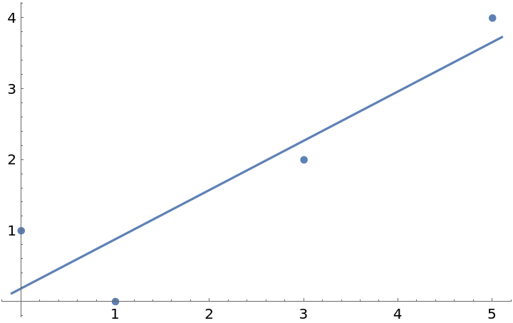

Plot two fits:

In[4]:=

data = {{0, 1}, {1, 0}, {3, 2}, {5, 4}};
data2 = {{0, 3}, {1, 4}, {3, 4}, {5, 6}};
lm = LinearModelFit[data, x, x];
lm2 = LinearModelFit[data2, x, x];
ResourceFunction["FittedModelPlot"][{lm, lm2}]

Out[8]=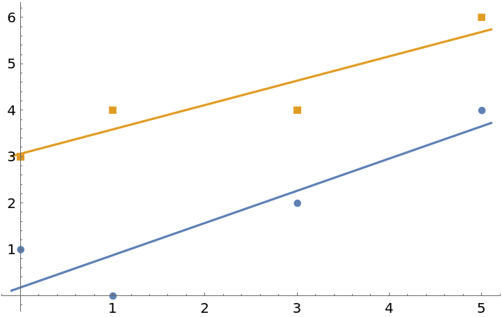

Style the plot and add a legend:

In[9]:=

data = {{0, 5}, {1, 2}, {3, 2}, {5, 1}};
data2 = {{0, 3}, {1, 4}, {3, 4}, {5, 6}};
lm = LinearModelFit[data, x, x];
lm2 = LinearModelFit[data2, x, x];
ResourceFunction[
"FittedModelPlot"][<|"Data 1" -> lm, "Data 2" -> lm2|>,
Frame -> True, PlotStyle -> Directive[Dashed, Thick], PlotTheme -> "VibrantColor"]

Out[13]=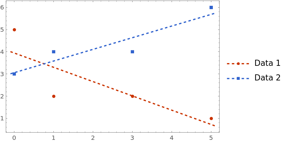

Supply the data to FittedModelPlot directly:

In[14]:=

data = {{0, 5}, {1, 2}, {3, 2}, {5, 1}};
data2 = {{0, 3}, {1, 4}, {3, 4}, {5, 6}};
ResourceFunction["FittedModelPlot"][
<|"Data 1" -> data, "Data 2" -> data2|>, x, x,
Frame -> True, PlotStyle -> Directive[Dashed, Thick], PlotTheme -> "VibrantColor", "ErrorBands" -> True
]

Out[16]=

Scope (2)

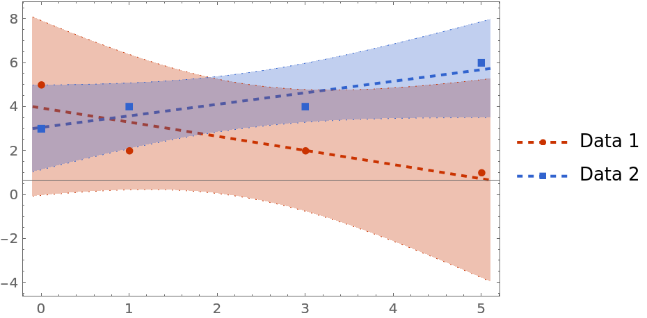Specify labels and callouts via wrappers, and specify that the callout should be attached to the fit line:

In[17]:=

data = {{0, 1}, {1, 0}, {3, 2}, {5, 4}};
data2 = {{0, 3}, {1, 4}, {3, 4}, {5, 6}};
ResourceFunction["FittedModelPlot"][
<|"Data 1" -> Callout[data, "Some callout", {Fit, 2}], "Data 2" -> Labeled[data2, "Some label", {Scaled@1, Before}]|>,
x,
x,
Frame -> True
]

Out[19]=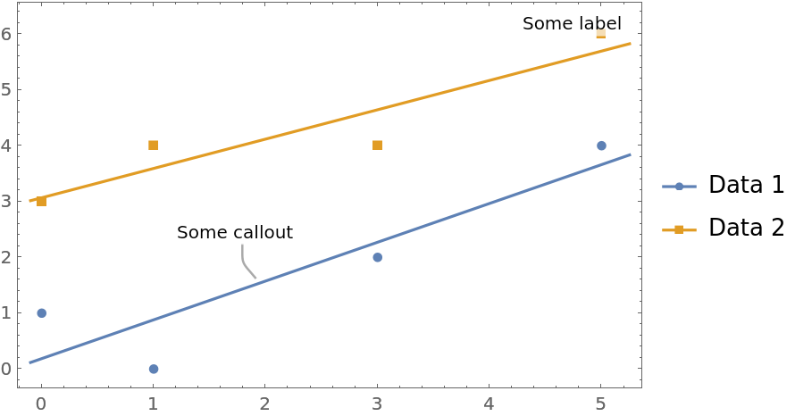

Plot the fit over a wider range:

In[20]:=

data = {{0, 1}, {1, 0}, {3, 2}, {5, 4}};
lm = LinearModelFit[data, x, x];
ResourceFunction["FittedModelPlot"][lm, {-2, 8}, Frame -> True]

Out[22]=

Options (5)

ErrorBands (3)

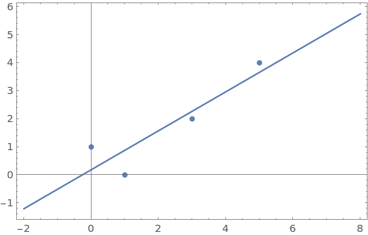With the default setting "ErrorBands"→False, no error bands are plotted:

In[23]:=

Out[25]=

Add error bands to the plot:

In[26]:=

data = {{0, 1}, {1, 0}, {3, 2}, {5, 4}};
lm = LinearModelFit[data, x, x];
ResourceFunction["FittedModelPlot"][lm, "ErrorBands" -> True]

Out[28]=

The setting for ConfidenceLevel affects the error bands:

In[29]:=

data = {{0, 1}, {1, 0}, {3, 2}, {5, 4}};
lm = LinearModelFit[data, x, x];
ResourceFunction["FittedModelPlot"][lm, ConfidenceLevel -> 0.7, "ErrorBands" -> True]

Out[31]=

LegendFunction (2)

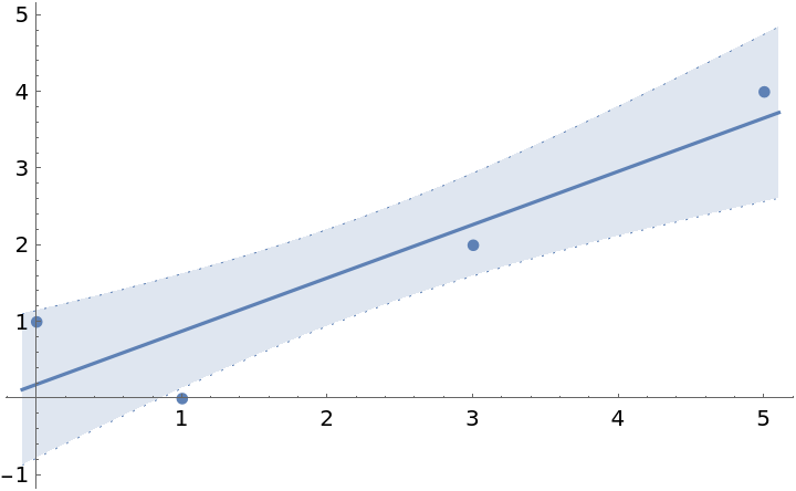With the default setting LegendFunction→Automatic, the legend is effectively generated from the PlotLegends setting:

In[32]:=

$data = { {{0, 2}, {1, 1}, {3, 3}, {5, 7}, {6, 5}, {7, 8}}, {{0, 1}, {1, 0}, {3, 2}, {5, 4}, {6, 4}, {7, 5}} }; ResourceFunction["FittedModelPlot"][data, Log[a + b x^2], {a, b}, x, PlotLegends -> {"A", "B"}]$

Out[33]=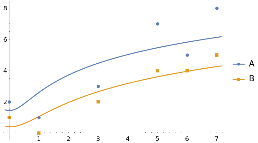

Give a function to compute the legend from the FittedModel[…] expressions:

In[34]:=

$data = { {{0, 2}, {1, 1}, {3, 3}, {5, 7}, {6, 5}, {7, 8}}, {{0, 1}, {1, 0}, {3, 2}, {5, 4}, {6, 4}, {7, 5}} }; ResourceFunction["FittedModelPlot"][data, Log[a + b x^2], {a, b}, x, LegendFunction -> Map[#["BestFit"] &]]$

Out[35]=

Properties and Relations (1)

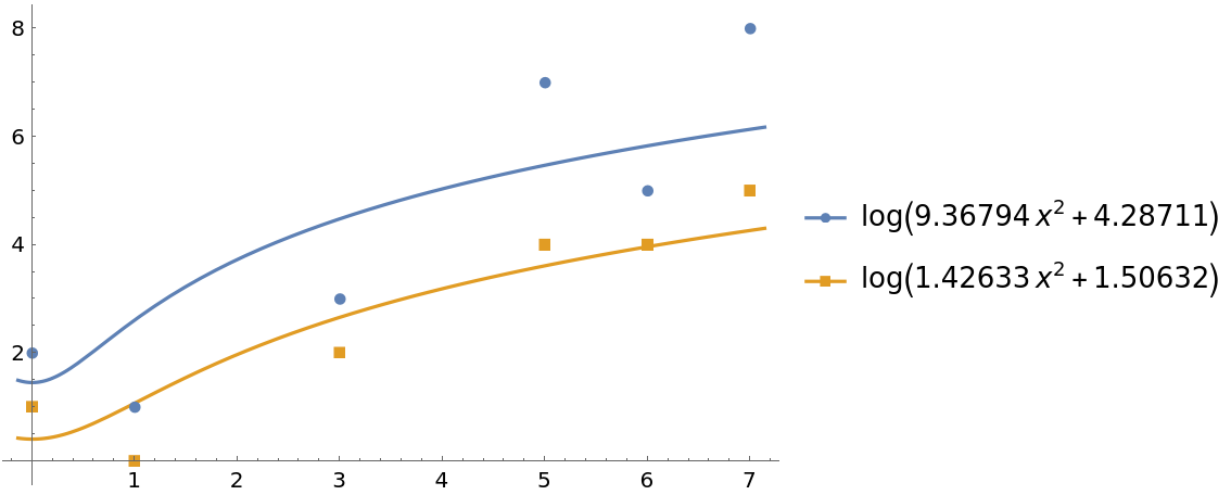FittedModelPlot can be recreated using a combination of ListPlot and Plot:

In[36]:=

$data = {{0, 1}, {1, 0}, {3, 2}, {5, 4}, {6, 4}, {7, 5}}; nlm = NonlinearModelFit[data, Log[a + b x^2], {a, b}, x]; Show[ListPlot[data], Plot[nlm[x], {x, 0, 7}], Frame -> True]$

Out[38]=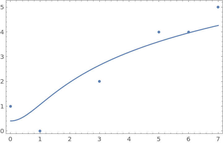

In[39]:=

Out[39]=

Neat Examples (2)

Generate some noisy data for three normal distributions:

In[40]:=

$SeedRandom[2] amp = RandomReal[{1, 3}, 3]; x0 = RandomReal[{-3, 3}, 3]; \[Sigma] = RandomReal[{0.5, 1}, 3]; data = MapThread[ Table[{x, # Exp[-(x - #2)^2/(2 #3^2)]}, {x, Subdivide[-4, 4, 30]}] &, {amp, x0, \[Sigma]}]; data += RandomReal[{-0.3, 0.3}, {3, 31, 2}];$

Plot the data together with their fits:

In[41]:=

$ResourceFunction["FittedModelPlot"][data, a Exp[-(x - b)^2/(2 c^2)], {a, b, c}, x, PlotTheme -> {"Detailed", "NeonColor", "ThickLines", "OpenMarkersThick"}, "ErrorBands" -> True, ConfidenceLevel -> 0.999, PlotRange -> All, PlotLegends -> {"A", "B", "C"} ]$

Out[41]=

Publisher

Lukas Lang

Version History

2.0.0 – 11 November 2020
1.0.0 – 25 September 2020

Related Resources

Author Notes

Changes from version 1.0.0 to 1.1.0:

Fixed the discrepancy between the plot markers used in the legend and in the plot.

Removed the example using style wrappers due to a bug in ListPlot failing to apply those styles to PlotMarkers.

Ensured that Labeled and Callout wrappers are only applied once, and added a way to control to which part they should be attached.

License Information

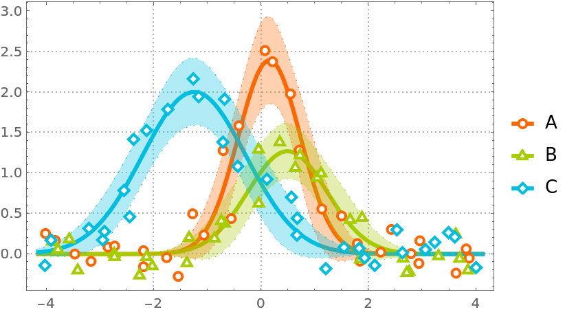This work is licensed under a Creative Commons Attribution 4.0 International License