Wolfram Function Repository
Instant-use add-on functions for the Wolfram Language
Function Repository Resource:
Convert a 3D curve into a parametrized tube
ResourceFunction["CurveTube"][c,t,r,θ] gives the parametrized circular tube with radius r and cross sectional angle θ centered on the curve c with parameter t. | |
ResourceFunction["CurveTube"][c1,c2,t,r,θ] gives the parametrized tube whose cross section is similar to c2 with effective radius r and cross sectional angle θ centered on the curve c1 with parameter t. |
Compute the parametrization for a helical tube:
| In[1]:= |
| Out[1]= |
Plot the tube:
| In[2]:= | ![ParametricPlot3D[
Evaluate[
ResourceFunction["CurveTube"][
Entity["SpaceCurve", "Helix"][
EntityProperty["SpaceCurve", "ParametricEquations"]][2., .5][t],
t, .5, \[Theta]]], {t, 0, 4 \[Pi]}, {\[Theta], 0, 2 \[Pi]}]](https://www.wolframcloud.com/obj/resourcesystem/images/579/5798a7df-ad00-450b-a036-785f983610d9/7ac450710077c7a7.png) |
| Out[2]= | 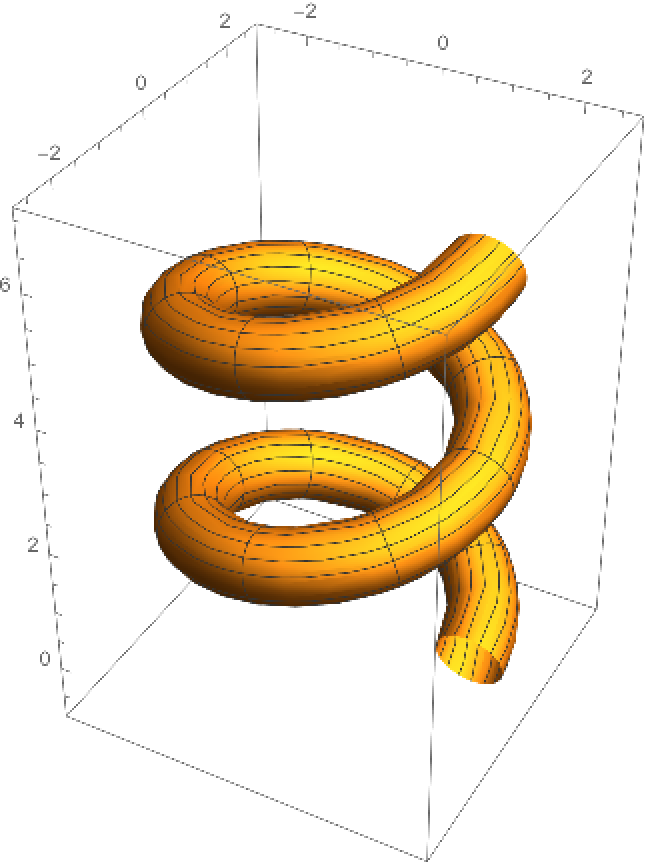 |
Make a tube from a torus knot curve:
| In[3]:= |
| In[4]:= | ![ParametricPlot3D[
Evaluate[
ResourceFunction["CurveTube"][torusknot[8, 3, 5][2, 5][t], t, 1, \[Theta]]], {t, 0, 2 \[Pi]}, {\[Theta], 0, 2 \[Pi]}, PlotPoints -> 60]](https://www.wolframcloud.com/obj/resourcesystem/images/579/5798a7df-ad00-450b-a036-785f983610d9/6bfb98732f9f25cd.png) |
| Out[4]= | 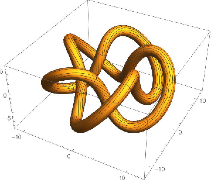 |
Make a helix tube using a variant of a nephroid as a cross section:
| In[5]:= |
| In[6]:= |
| Out[6]= | 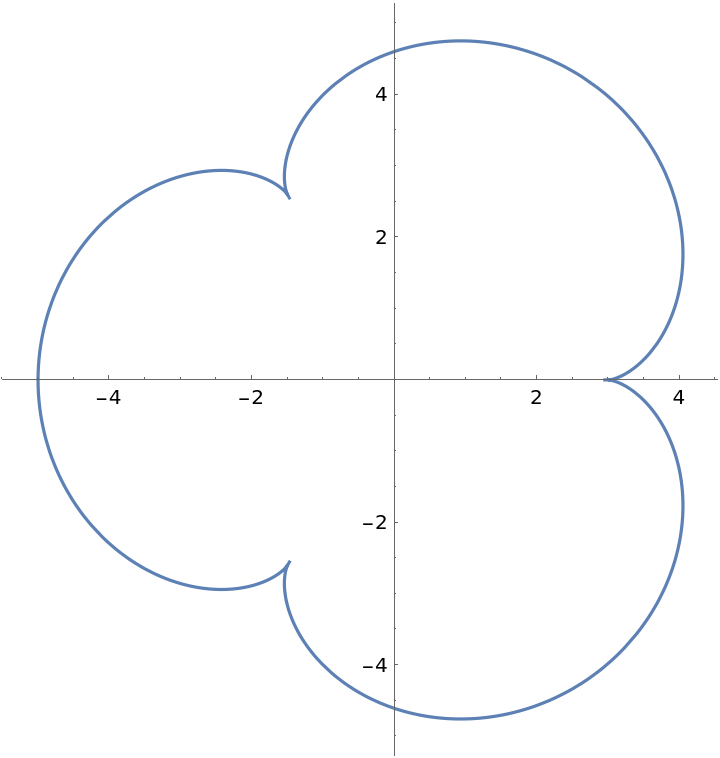 |
| In[7]:= | ![ct = ResourceFunction["CurveTube"][
Entity["SpaceCurve", "Helix"][
EntityProperty["SpaceCurve", "ParametricEquations"]][1, 1/2][t],
nephroid[1][t], t, r, \[Theta]] // Chop](https://www.wolframcloud.com/obj/resourcesystem/images/579/5798a7df-ad00-450b-a036-785f983610d9/5b873b7e4cbc816f.png) |
| Out[7]= |  |
| In[8]:= |
| Out[8]= | 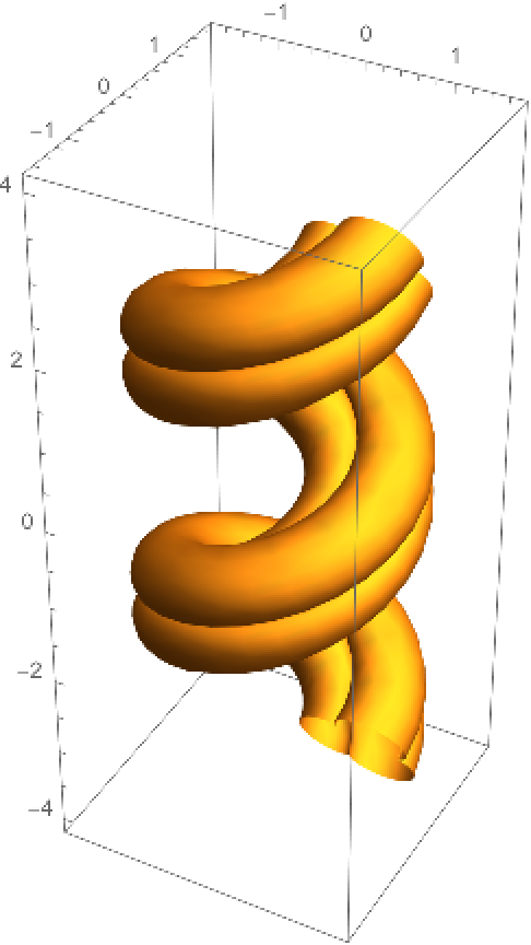 |
Take the normal and binormal vectors from the Frenet-Serret system for a helix:
| In[9]:= | ![fss = FullSimplify[
PowerExpand[
Rest[FrenetSerretSystem[
Entity["SpaceCurve", "Helix"][
EntityProperty["SpaceCurve", "ParametricEquations"]][a, b][
t], t][[2]]]]]](https://www.wolframcloud.com/obj/resourcesystem/images/579/5798a7df-ad00-450b-a036-785f983610d9/2e9da5b74ff8e0e4.png) |
| Out[9]= |
The parametrization for the curve tube for a helix is:
| In[10]:= | ![Entity["SpaceCurve", "Helix"][
EntityProperty["SpaceCurve", "ParametricEquations"]][a, b][t] + r (-Cos[\[Theta]] fss[[1]] + Sin[\[Theta]] fss[[2]]) // FullSimplify](https://www.wolframcloud.com/obj/resourcesystem/images/579/5798a7df-ad00-450b-a036-785f983610d9/0b547b94ed7ac24d.png) |
| Out[10]= |
This is the same as given by CurveTube:
| In[11]:= |
| Out[11]= |
Something similar can be done with Tube:
| In[12]:= | ![Graphics3D[
Tube[BSplineCurve[
Table[Entity["SpaceCurve", "Helix"][
EntityProperty["SpaceCurve", "ParametricEquations"]][2., .5][
t], {t, 0, 4 \[Pi], 4 \[Pi]/20}]], .25]]](https://www.wolframcloud.com/obj/resourcesystem/images/579/5798a7df-ad00-450b-a036-785f983610d9/7cde49c71f7cc547.png) |
| Out[12]= | 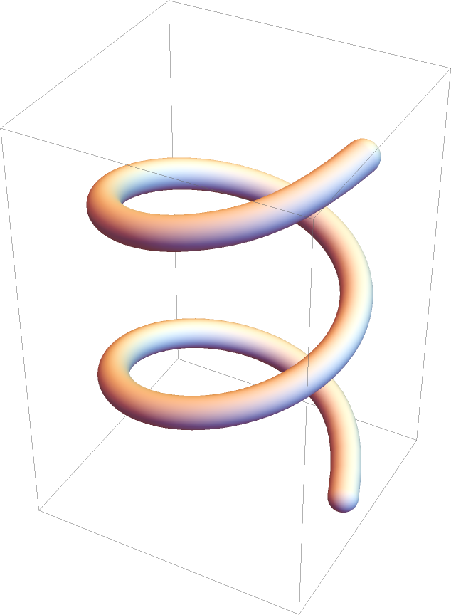 |
This work is licensed under a Creative Commons Attribution 4.0 International License