Wolfram Function Repository
Instant-use add-on functions for the Wolfram Language
Function Repository Resource:
Get the parametrization of a seashell surface
ResourceFunction["SeaShellSurface"][γ,r,{t,θ}] gives a parametrization of a seashell surface γ with variable radius r and parameters t and θ. |
The parametrization of a helix:
| In[1]:= |
| Out[1]= |
Get the complete parametrization of a helical seashell surface:
| In[2]:= |
| Out[2]= |  |
Plot the surface:
| In[3]:= | ![ParametricPlot3D[
Evaluate[
ResourceFunction["SeaShellSurface"][
helix[1, .6][t], .1, {t, \[Theta]}]], {t, \[Pi]/4, 5 \[Pi]}, {\[Theta], 0, 2 \[Pi]}, Boxed -> False, Axes -> None, PlotPoints -> 50, ViewPoint -> Front]](https://www.wolframcloud.com/obj/resourcesystem/images/afb/afb4ebd6-277e-4ca8-8534-89d79cdd4db4/28377cd3bae0f5e2.png) |
| Out[3]= | 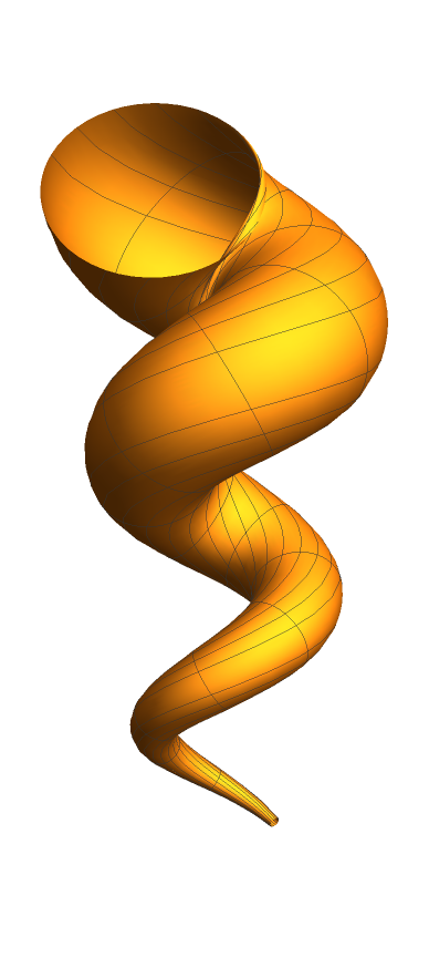 |
Visualize the plot using Manipulate:
| In[4]:= | ![Manipulate[
ParametricPlot3D[
Evaluate[
ResourceFunction["SeaShellSurface"][helix[a, b][t], c, {t, \[Theta]}]], {t, \[Pi]/4, 5 \[Pi]}, {\[Theta], 0, 2 \[Pi]},
Boxed -> False, Axes -> None, MaxRecursion -> 3, PlotStyle -> Opacity[op], Mesh -> None], {{a, 1.8}, .5, 2.}, {{b, .2}, .2, 2.}, {{c, .3}, .04, 1.}, {{op, .5}, .2, 1}]](https://www.wolframcloud.com/obj/resourcesystem/images/afb/afb4ebd6-277e-4ca8-8534-89d79cdd4db4/63f145dcabe6b981.png) |
| Out[4]= | 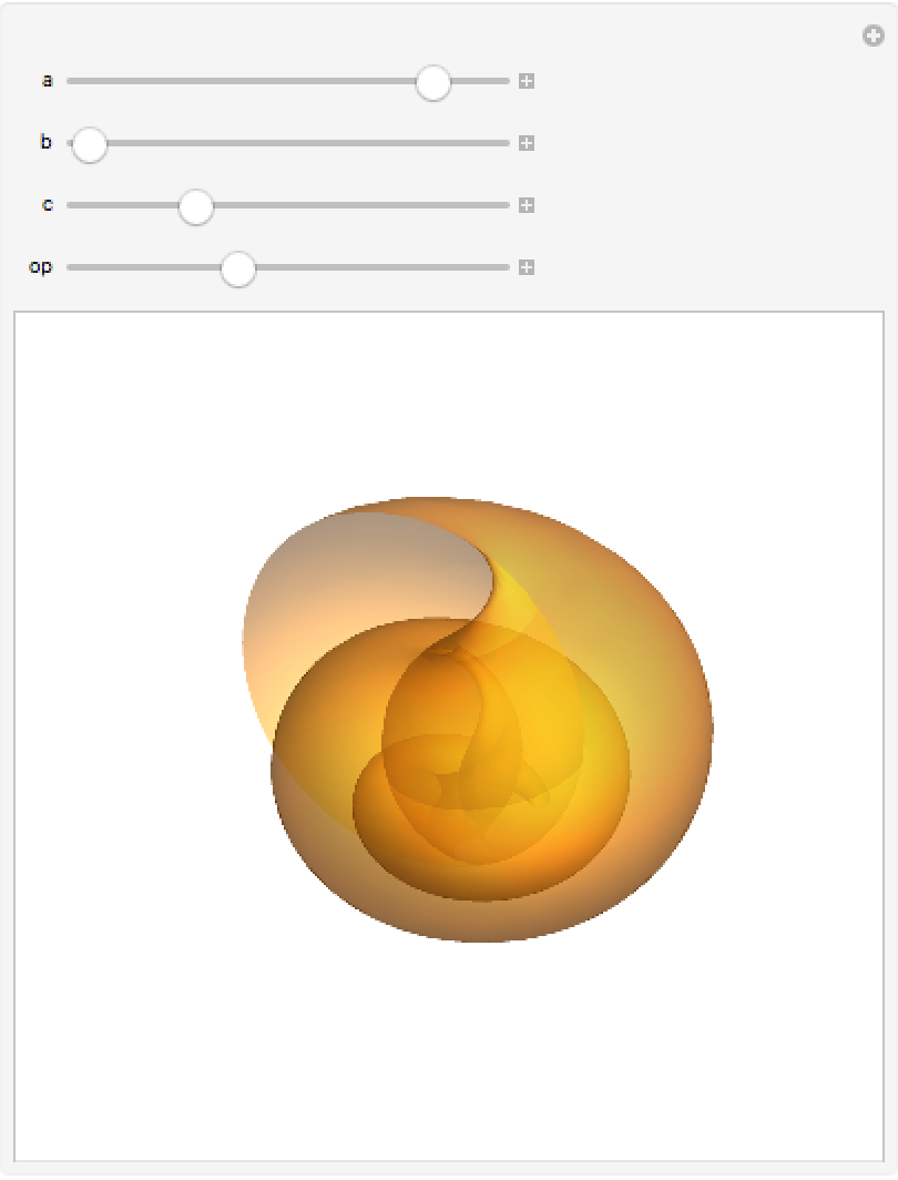 |
Create a dynamic version using DynamicModule in conjunction with Evaluate:
| In[5]:= | ![DynamicModule[{a = 1.836`, b = 0.2`, c = 0.32499999999999996`}, ParametricPlot3D[
Evaluate[
ResourceFunction["SeaShellSurface"][helix[a, b][t], c, {t, \[Theta]}]], {t, \[Pi]/4, 5 \[Pi]}, {\[Theta], 0, 2 \[Pi]},
Boxed -> False, Axes -> None, MaxRecursion -> 3]]](https://www.wolframcloud.com/obj/resourcesystem/images/afb/afb4ebd6-277e-4ca8-8534-89d79cdd4db4/6bf8bd1bc399139c.png) |
| Out[5]= | 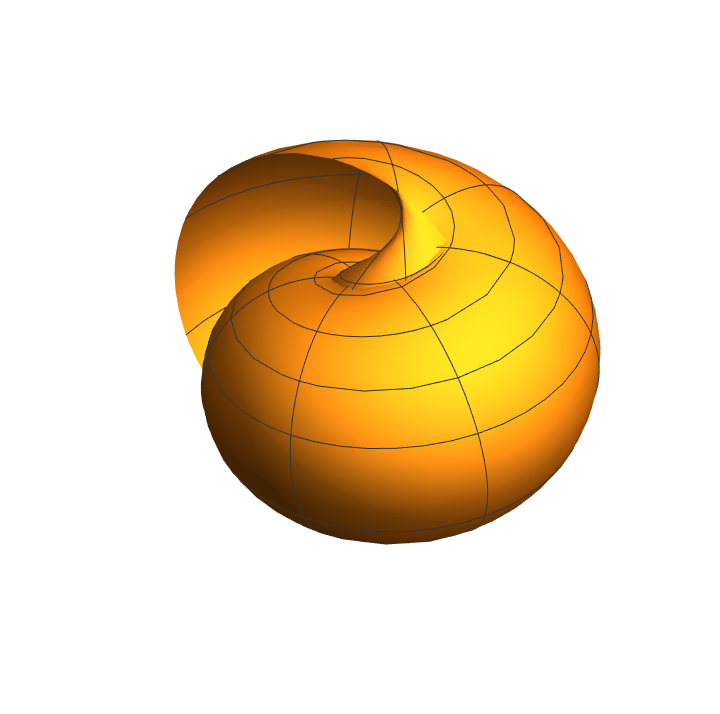 |
Nordstrand's version:
| In[6]:= | ![g = With[{a = 0.2, b = 1, c = 0.1, n = 2}, ParametricPlot3D[{((1 - v/(2 \[Pi])) (1 + Cos[u]) + c) Cos[
n v], ((1 - v/(2 \[Pi])) (1 + Cos[u]) + c) Sin[n v], (b v)/(
2 \[Pi]) + a Sin[u] (1 - v/(2 \[Pi]))}, {u, 0, 2 \[Pi]}, {v, 0, 2 \[Pi]}, Boxed -> False, PlotPoints -> {25, 100}, Axes -> False, PlotRange -> All, ViewPoint -> {0, -2, 0.2}, BoxRatios -> {1, 1, 1}]]](https://www.wolframcloud.com/obj/resourcesystem/images/afb/afb4ebd6-277e-4ca8-8534-89d79cdd4db4/517787fa26ce077f.png) |
| Out[6]= | 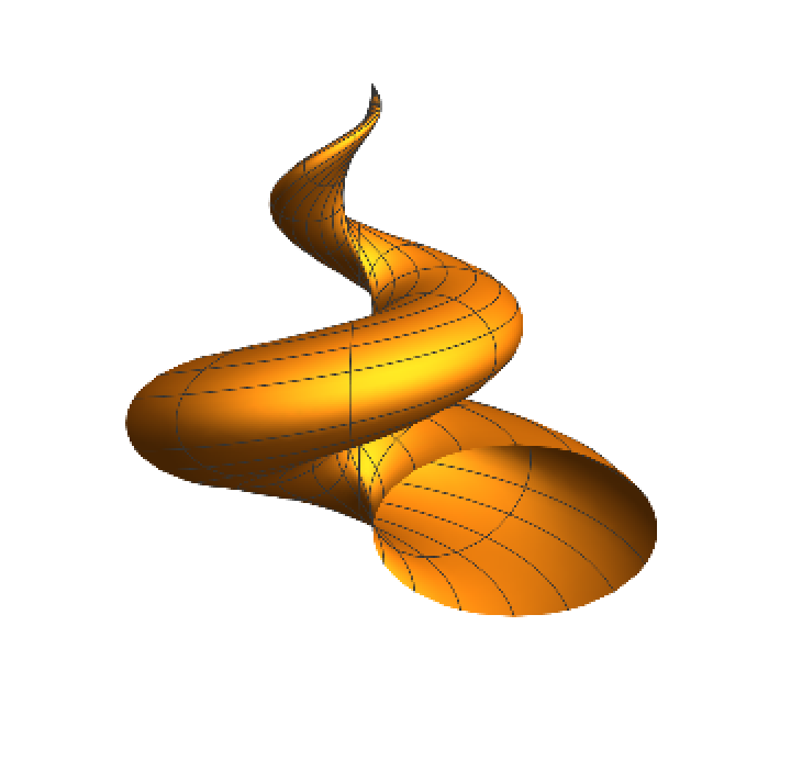 |
Upright conical spiral (models by S. Dickson):
| In[7]:= | ![ParametricPlot3D[{2 (1 - Exp[u/(6 \[Pi])]) Cos[u] Cos[v/2]^2, 2 (-1 + Exp[u/(6 \[Pi])]) Sin[u] Cos[v/2]^2, 1 - Exp[u/(3 \[Pi])] - Sin[v] + Exp[u/(6 \[Pi])] Sin[v]}, {u, 0, 6 \[Pi]}, {v, 0, 2 \[Pi]}, Boxed -> False, PlotPoints -> {100, 25}, Axes -> False, PlotRange -> All, ViewPoint -> {0, 2, 1}]](https://www.wolframcloud.com/obj/resourcesystem/images/afb/afb4ebd6-277e-4ca8-8534-89d79cdd4db4/21f0bed134272853.png) |
| Out[7]= | 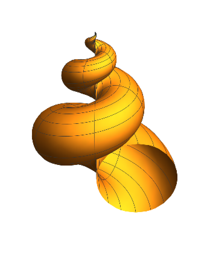 |
Upright conical spiral with gradual slope:
| In[8]:= |
| In[9]:= |
| In[10]:= |
| In[11]:= |
| Out[11]= | 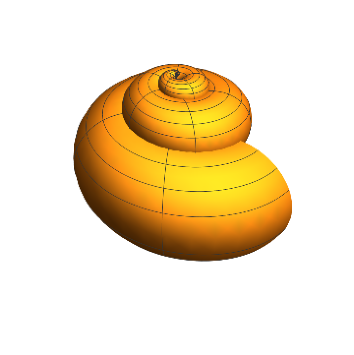 |
Cross-section of flat conical spiral:
| In[12]:= |
| In[13]:= |
| In[14]:= |
| In[15]:= |
| Out[15]= | 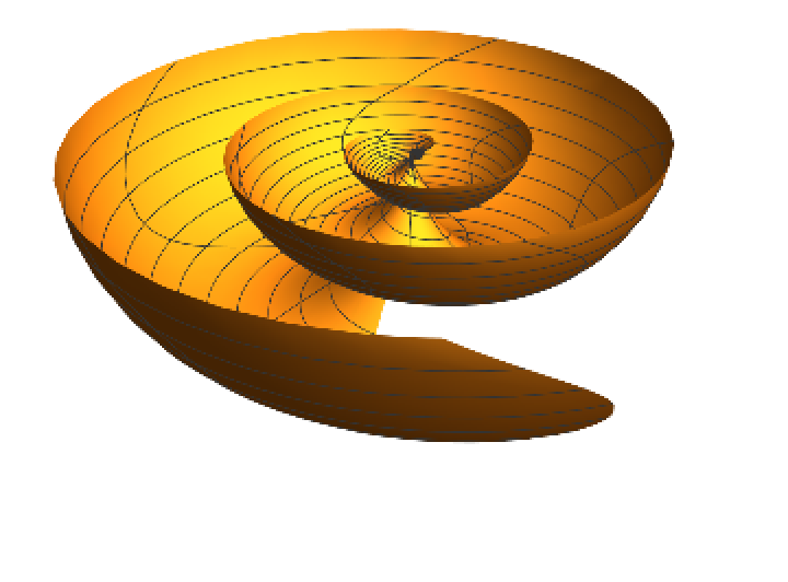 |
Wolfram's model:
| In[16]:= | ![With[{a = 1.2, b = 2, c = 1.5, d = 1, e = 1.2}, ParametricPlot3D[
a^t {Cos[
t] (1 + c (Cos[e] Cos[\[Theta]] + (d Sin[e]) Sin[\[Theta]])), Sin[t] (1 + c (Cos[e] Cos[\[Theta]] + (d Sin[e]) Sin[\[Theta]])), b + c (Cos[\[Theta]] Sin[
e] - (d Cos[
e]) Sin[\[Theta]])}, {\[Theta], -\[Pi], \[Pi]}, {t, -25, 0}, PlotPoints -> 80,
PlotStyle -> Directive[Opacity[1 - .5], Lighter[Yellow, 0.3], Specularity[White, 10]], Axes -> None, ViewPoint -> {1, 1, -3}, Boxed -> False, PlotRange -> All, Mesh -> None]]](https://www.wolframcloud.com/obj/resourcesystem/images/afb/afb4ebd6-277e-4ca8-8534-89d79cdd4db4/14ad5025aeeb6b90.png) |
| Out[16]= | 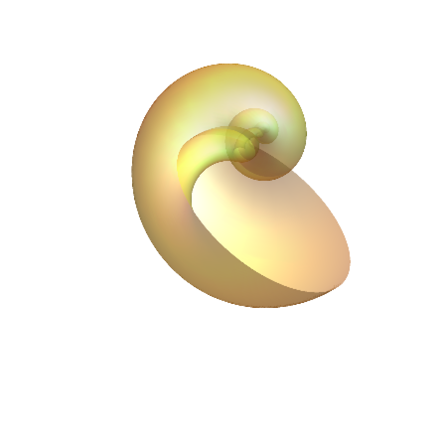 |
This work is licensed under a Creative Commons Attribution 4.0 International License