Wolfram Function Repository
Instant-use add-on functions for the Wolfram Language
Function Repository Resource:
Visualize the directional derivative in a 3D plot
ResourceFunction["DirectionalDerivativePlot3D"][f,{x,xmin,xmax},{y,ymin,ymax},pt,v]]] returns a plot of f along with a plot of the directional derivative vector at the point pt in the direction of the vector v. Several points and/or vectors can be given in a list. |
| "ArrowSize" | Medium | size of the arrowhead |
| "BaseVectorPosition" | Automatic | determines the position of the base vector if drawn |
| "DrawBaseVector" | False | whether to draw the base vector |
| "DrawGraph" | True | whether to include the plot of the surface |
| "DrawPlane" | False | whether to include the plane determining the section |
| "PointStyle" | PointSize[Large] | graphics directive to specify the style for the point(s) |
| "PrintDisplay" | False | whether to print the value of the directional derivative |
| "SectionStyle" | {{Tube[0.01],Black}} | style for the section determined by the direction vector |
| "UseLimit" | False | whether to use the limit definition to calculate the directional derivative |
| "VectorStyle" | {{Thickness[Medium],Red}} | graphics directive to specify the style for the vector(s) |
Visualize a directional derivative:
| In[1]:= |
| Out[1]= | 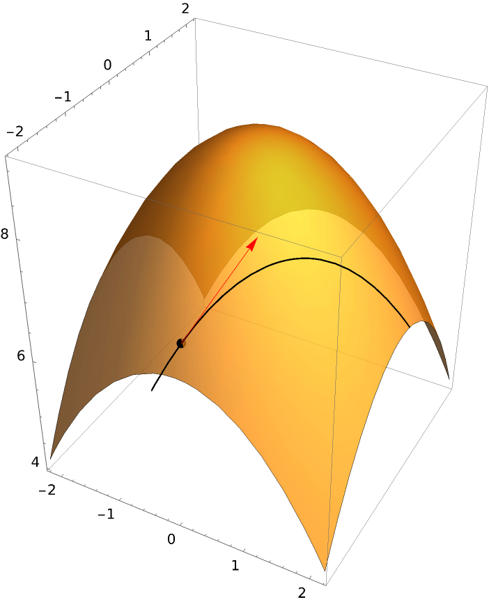 |
Suppress drawing the section curve:
| In[2]:= | ![ResourceFunction["DirectionalDerivativePlot3D"][
9 - x^2/2 - y^2/2, {x, -2.2, 2.2}, {y, -2.2, 2.2}, {0, -2}, {Cos[\[Pi]/4], Sin[\[Pi]/4]}, "SectionStyle" -> Tube[0]]](https://www.wolframcloud.com/obj/resourcesystem/images/ff7/ff77cfac-f65a-4b6e-8f93-5c43c2a95b29/47ba97686620eed7.png) |
| Out[2]= |  |
Plot using two direction vectors:
| In[3]:= | ![ResourceFunction["DirectionalDerivativePlot3D"][
9 - x^2/2 - y^2/2, {x, -2.2, 2.2}, {y, -2.2, 2.2}, {0, -2}, {{Cos[\[Pi]/4], Sin[\[Pi]/4]}, {1, 0}}]](https://www.wolframcloud.com/obj/resourcesystem/images/ff7/ff77cfac-f65a-4b6e-8f93-5c43c2a95b29/30639e2ddbe99dc2.png) |
| Out[3]= | 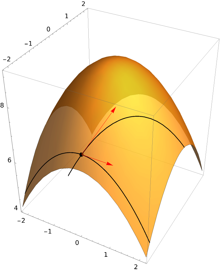 |
Include a print of the values of the directional derivatives:
| In[4]:= | ![ResourceFunction["DirectionalDerivativePlot3D"][
9 - x^2/2 - y^2/2, {x, -2.2, 2.2}, {y, -2.2, 2.2}, {0, -2}, {{Cos[\[Pi]/4], Sin[\[Pi]/4]}, {1, 0}}, "PrintDisplay" -> True]](https://www.wolframcloud.com/obj/resourcesystem/images/ff7/ff77cfac-f65a-4b6e-8f93-5c43c2a95b29/6452167e99154cbc.png) |
| Out[4]= |  |
Return just a print of the points and the directional derivatives:
| In[5]:= | ![ResourceFunction["DirectionalDerivativePlot3D"][
9 - x^2/2 - y^2/2, {x, -2.2, 2.2}, {y, -2.2, 2.2}, {0, -2}, {{Cos[\[Pi]/4], Sin[\[Pi]/4]}, {1, 0}}, "DrawGraph" -> False]](https://www.wolframcloud.com/obj/resourcesystem/images/ff7/ff77cfac-f65a-4b6e-8f93-5c43c2a95b29/5114754d83d49fa2.png) |
| Out[5]= |
Plot using two direction vectors and two points:
| In[6]:= | ![ResourceFunction["DirectionalDerivativePlot3D"][
9 - x^2/2 - y^2/2, {x, -2.2, 2.2}, {y, -2.2, 2.2}, {{0, -2}, {1, -1/2}}, {{Cos[\[Pi]/4], Sin[\[Pi]/4]}, {1, 0}}]](https://www.wolframcloud.com/obj/resourcesystem/images/ff7/ff77cfac-f65a-4b6e-8f93-5c43c2a95b29/1bb77e4a66055031.png) |
| Out[6]= |  |
If "DrawBaseVector" is set to True, then the vector determining the direction is plotted at the bottom of the plot:
| In[7]:= | ![ResourceFunction["DirectionalDerivativePlot3D"][
9 - x^2/2 - y^2/2, {x, -2.2, 2.2}, {y, -2.2, 2.2}, {{0, -2}, {1, 0}}, {Cos[\[Pi]/4], Sin[\[Pi]/4]}, "DrawBaseVector" -> True]](https://www.wolframcloud.com/obj/resourcesystem/images/ff7/ff77cfac-f65a-4b6e-8f93-5c43c2a95b29/115b80709c9a1555.png) |
| Out[7]= | 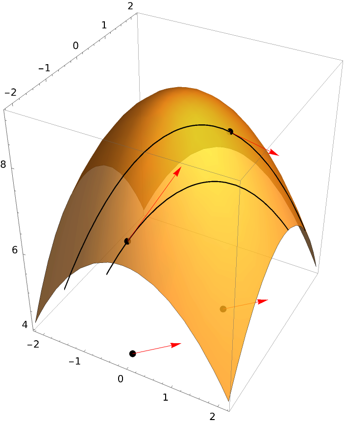 |
Include the plane determining the section along with the base vector in the plot:
| In[8]:= | ![ResourceFunction["DirectionalDerivativePlot3D"][
9 - x^2/2 - y^2/2, {x, -2.2, 2.2}, {y, -2.2, 2.2}, {0, -2}, {Cos[\[Pi]/4], Sin[\[Pi]/4]}, "PointStyle" -> PointSize[Large], "DrawBaseVector" -> True, "DrawPlane" -> True]](https://www.wolframcloud.com/obj/resourcesystem/images/ff7/ff77cfac-f65a-4b6e-8f93-5c43c2a95b29/1f6e1c3ebef81b52.png) |
| Out[8]= | 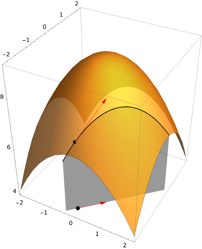 |
The option "BaseVectorPosition" allows the vector to be plotted in any horizontal plane:
| In[9]:= | ![ResourceFunction["DirectionalDerivativePlot3D"][
9 - x^2/2 - y^2/2, {x, -2.2, 2.2}, {y, -2.2, 2.2}, {0, -2}, {Cos[\[Pi]/4], Sin[\[Pi]/4]}, "DrawBaseVector" -> True, "BaseVectorPosition" -> (9 - x^2/2 - y^2/2 /. {x -> 0, y -> -2})]](https://www.wolframcloud.com/obj/resourcesystem/images/ff7/ff77cfac-f65a-4b6e-8f93-5c43c2a95b29/586addcf77c4bd2e.png) |
| Out[9]= |  |
Set a style for the vectors:
| In[10]:= | ![ResourceFunction["DirectionalDerivativePlot3D"][
Sin[\[Pi] x y], {x, -1, 1}, {y, -1, 1}, {1/2, 1/2}, {{1, 2}, {1, 0}},
"PointStyle" -> {{PointSize[.025], Green}}, PlotRange -> All, VectorStyle -> {{Thickness[Large], Red}, Green}, PlotStyle -> Opacity[.6], Mesh -> None]](https://www.wolframcloud.com/obj/resourcesystem/images/ff7/ff77cfac-f65a-4b6e-8f93-5c43c2a95b29/53f92329498038b8.png) |
| Out[10]= | 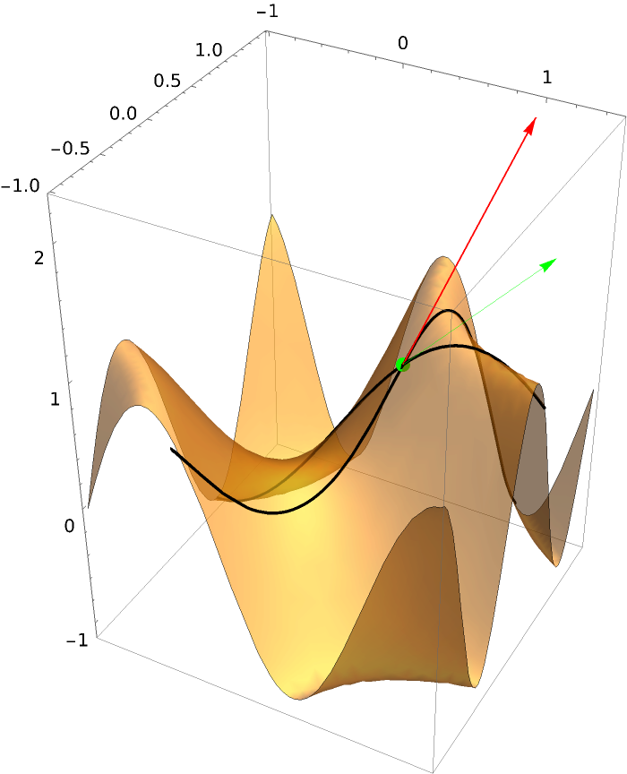 |
Add the base vectors and lower their position:
| In[11]:= | ![ResourceFunction["DirectionalDerivativePlot3D"][
Sin[\[Pi] x y], {x, -1, 1}, {y, -1, 1}, {1/2, 1/2}, {{1, 2}, {1, 0}},
"PointStyle" -> {{PointSize[.025], Green}}, PlotRange -> All, VectorStyle -> {Red, Green}, PlotStyle -> Opacity[.6], Mesh -> None, "DrawBaseVector" -> True, "BaseVectorPosition" -> -3]](https://www.wolframcloud.com/obj/resourcesystem/images/ff7/ff77cfac-f65a-4b6e-8f93-5c43c2a95b29/7c130aa0f3d0ea94.png) |
| Out[11]= | 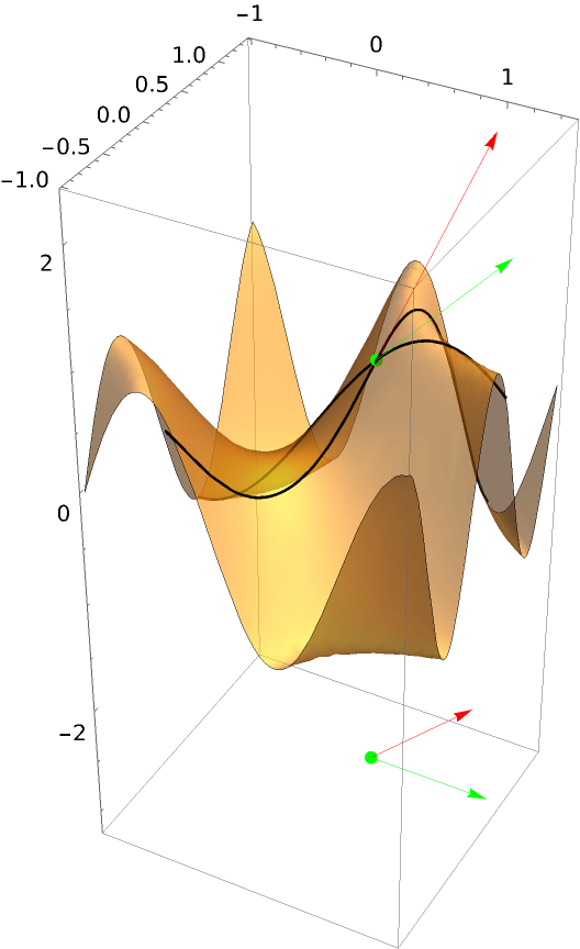 |
A function requiring both "UseLimit” and ResourceFunction["UseRealRoots"]:
| In[12]:= | ![ResourceFunction["DirectionalDerivativePlot3D"][(x y^2)^(
1/3), {x, -1.2, 1.2}, {y, -1.2, 1.2}, {0, 0}, {-1, -1}, "UseLimit" -> True, Mesh -> None, PlotStyle -> Opacity[.5], "DrawBaseVector" -> True, "PrintDisplay" -> True] // ResourceFunction["UseRealRoots"]](https://www.wolframcloud.com/obj/resourcesystem/images/ff7/ff77cfac-f65a-4b6e-8f93-5c43c2a95b29/1f1ef9020f17ad89.png) |
| Out[12]= | 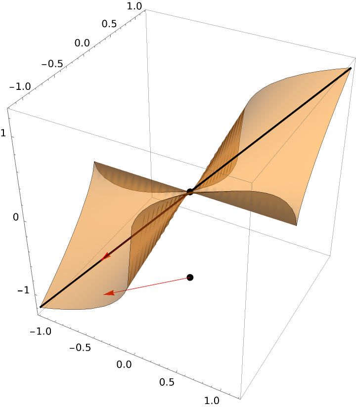 |
Without using ResourceFunction["UseRealRoots"]:
| In[13]:= | ![Quiet[ResourceFunction["DirectionalDerivativePlot3D"][(x y^2)^(
1/3), {x, -1.2, 1.2}, {y, -1.2, 1.2}, {0, 0}, {-1, -1}, Mesh -> None, PlotStyle -> Opacity[.5], "DrawBaseVector" -> True, "PrintDisplay" -> True]]](https://www.wolframcloud.com/obj/resourcesystem/images/ff7/ff77cfac-f65a-4b6e-8f93-5c43c2a95b29/09f975c5e48f2e8c.png) |
| Out[13]= | 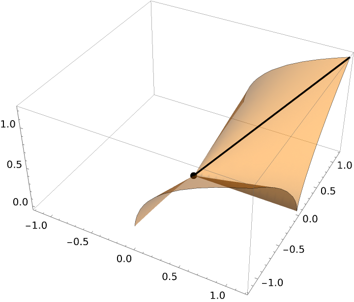 |
Without using the option "UseLimit":
| In[14]:= | ![Quiet[ResourceFunction["DirectionalDerivativePlot3D"][(x y^2)^(
1/3), {x, -1.2, 1.2}, {y, -1.2, 1.2}, {0, 0}, {-1, -1}, Mesh -> None, PlotStyle -> Opacity[.5], "DrawBaseVector" -> True, "PrintDisplay" -> True] // ResourceFunction["UseRealRoots"]]](https://www.wolframcloud.com/obj/resourcesystem/images/ff7/ff77cfac-f65a-4b6e-8f93-5c43c2a95b29/744977959e5fe02d.png) |
| Out[14]= | 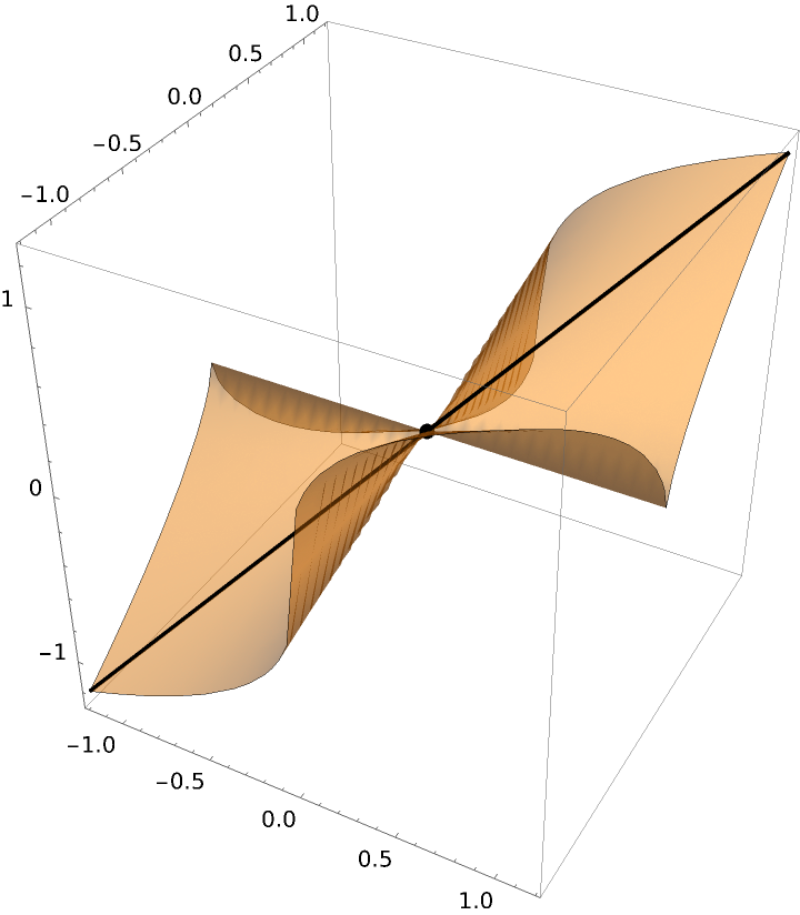 |
Another function requiring the option "UseLimit” and ResourceFunction["UseRealRoots"]:
| In[15]:= | ![(* Evaluate this cell to get the example input *) CloudGet["https://www.wolframcloud.com/obj/8e7b4e59-2d68-4788-a2f0-e4d00c6c8936"]](https://www.wolframcloud.com/obj/resourcesystem/images/ff7/ff77cfac-f65a-4b6e-8f93-5c43c2a95b29/67d0af02d1a7bba0.png) |
| Out[16]= | 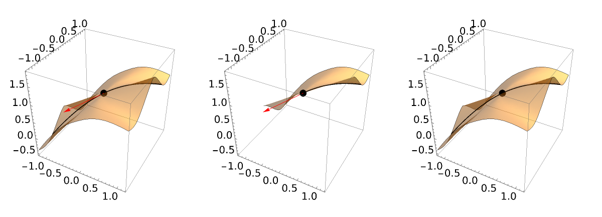 |
This work is licensed under a Creative Commons Attribution 4.0 International License