Basic Examples (4) 

The closure fills in missing elements within the range:

In[1]:=

Out[1]=

A convex set is a fixed point. It returns itself:

In[2]:=

Out[2]=

The closure of a singleton is the singleton itself:

In[3]:=

Out[3]=

Applied to a non-contiguous parent set:

In[4]:=

Out[4]=

Scope (3) 

Works with rational elements:

In[5]:=

Out[5]=

Works with strings under lexicographic order:

In[6]:=

Out[6]=

Works with symbolic heads that have a canonical ordering:

In[7]:=

Out[7]=

Options (3) 

The default value of "ComparisonFunction" is LessEqual:

In[8]:=

Out[8]=

Use GreaterEqual to compute the closure under the reverse order:

In[9]:=

Out[9]=

A custom comparison function. Closure under order by string length:

In[10]:=

Out[10]=

Applications (3) 

Find intermediate stations between two stops on a Mexico City Metro line, using positional ordering rather than alphabetical order via a custom index-based comparison:

In[11]:=

Out[11]=

Determine the contiguous range of monthly periods between two known events in a fiscal calendar:

In[12]:=

Out[12]=

The function reconstructs the full sequence of monthly periods between the two given dates, ensuring interval completeness within the fiscal calendar.

Extract all rows in a dataset whose key falls between two boundary values:

In[13]:=

Out[13]=

Properties and Relations (6) 

Idempotence. Applying the closure twice yields the same result:

In[14]:=

Out[14]=

A subset is convex if and only if it equals its closure:

In[15]:=

Out[15]=

The closure equals the subset joined with its defect (disjoint union):

In[16]:=

Out[16]=

The result of OrderConvexClosure always satisfies OrderConvexQ:

In[17]:=

Out[17]=

Extensiveness. The closure contains the original subset:

In[18]:=

Out[18]=

Monotonicity. If , then :

In[19]:=

Out[19]=

Possible Issues (1) 

OrderConvexClosure does not verify . If subset contains elements absent from parentSet, the closure is computed based on the range of subset but filtered from parentSet only. The function is designed for total orders only. For partial orders, the interval characterization does not hold. When using a custom "ComparisonFunction", the function must be a valid total preorder: reflexive, transitive, and total. Passing a non-transitive relation yields undefined behaviour. If subset has elements not in parent set, they act as bounds but do not appear in the output:

In[20]:=

Out[20]=

Neat Examples (4) 

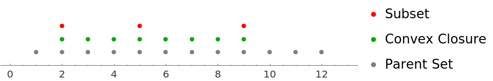
Visualize the closure on a number line. Red points show the original subset. Green marks the convex closure:

In[21]:=

Out[21]=

Enumerate all distinct closures obtainable from 2-element subsets of {1,…,8}:

In[22]:=

Out[22]=

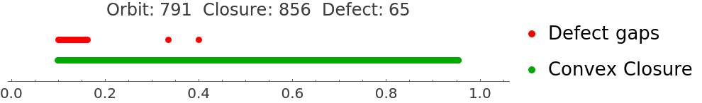
Fractal structure of the logistic map attractor. Discretize the orbit at r = 3.82 on a grid of resolution 0.001. Compare the orbit with its convex closure. The difference is the convex defect. Its size reflects gaps in the Cantor-like attractor:

In[23]:=

Out[23]=

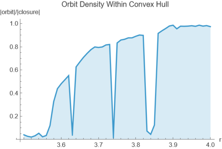
Sweep the parameter r from 3.5 to 4.0 and plot the size of the convex closure relative to the discretised orbit. As approaches 4, the attractor fills the interval and the ratio tends to 1:

In[24]:=

Out[24]=