Function Repository Resource:

LinearAlgebraMod

Source Notebook

Perform matrix operations over a finite field

Contributed by: Daniel Lichtblau

ResourceFunction["LinearAlgebraMod"][op,mat,p]

performs the operation op on matrix mat using prime modulus p.

ResourceFunction["LinearAlgebraMod"][LinearSolve,mat,rhs,p]

solves mat.x ==rhs for x, modulo p.

ResourceFunction["LinearAlgebraMod"][CharacteristicPolynomial,mat,t,p]

computes the characteristic polynomial for square matrix mat using t as the polynomial variable.

ResourceFunction["LinearAlgebraMod"][op]

represents an operator form that can be applied to matrix and modulus arguments.

ResourceFunction["LinearAlgebraMod"][op,p]

represents an operator form, with the operation and modulus both specified, that can be applied to a matrix.

Details and Options

When LinearSolve is the operation, a vector or second matrix must be given as the right-hand side.
The operation names can be given either as symbols or strings.
The modulus is 0 by default.
ResourceFunction["LinearAlgebraMod"] accepts an Extension option. It must be a univariate polynomial that is irreducible modulo the prime p, or irreducible over the rationals if the modulus is 0.
ResourceFunction["LinearAlgebraMod"] performs linear algebra over a finite field or an algebraic extension of the rationals, with an input matrix comprised of (not necessarily univariate) polynomial functions.

Examples

Basic Examples (11) 

Start with a 2×3 polynomial matrix in two variables, one of which will be used as an algebraic extension:

In[1]:=
mat = {{a^2 x + 1, 2 a x^2 + (a + 6) x + 5, (a^2 + a + 6) x + (3 a + 4)}, {(4 a + 2) x^2 + (a + 2) x + 3, (a^2 + 3 a + 3) x^2 + (a + 4) x + a, x + 1}};

The polynomial defining the extension:

In[2]:=
ext = a^3 + 5 a^2 + 3 a + 4;

Reduce to row echelon form over the finite extension field of integers mod 7 with 73=343 elements, given as :
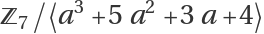
In[3]:=
ResourceFunction["LinearAlgebraMod"]["RowReduce", mat, 7, Extension -> ext]
Out[3]=

Compute the inverse of the submatrix comprised of the first two columns:

In[4]:=
inv = ResourceFunction["LinearAlgebraMod"]["Inverse", mat[[All, 1 ;; 2]], 7, Extension -> ext]
Out[4]=

Check that this inverse multiplied by mat gives the 2×2 identity matrix:

In[5]:=
Together[PolynomialMod[inv . mat[[All, 1 ;; 2]], {7, ext}], Modulus -> 7]
Out[5]=

Use the last column as a right-hand side for a matrix equation:

In[6]:=
sol = ResourceFunction["LinearAlgebraMod"]["LinearSolve", mat[[All, 1 ;; 2]], mat[[All, 3]], 7, Extension -> ext]
Out[6]=

Check the result:

In[7]:=
PolynomialMod[mat[[All, 1 ;; 2]] . sol - mat[[All, 3]], {7, ext}]
Out[7]=

Find a basis for the null space of the full matrix:

In[8]:=
nulls = ResourceFunction["LinearAlgebraMod"]["NullSpace", mat, 7, Extension -> ext]
Out[8]=

Check that it has only null vectors for mat:

In[9]:=
Together[PolynomialMod[mat . Transpose[nulls], {7, ext}], Modulus -> 7]
Out[9]=

Since there are three columns and the null space is generated by one vector, the rank must be 2:

In[10]:=
rank = ResourceFunction["LinearAlgebraMod"]["MatrixRank", mat, 7, Extension -> ext]
Out[10]=

Compute the characteristic polynomial for the matrix augmented by a row of ones:

In[11]:=
ResourceFunction["LinearAlgebraMod"]["CharacteristicPolynomial", Append[mat, {1, 1, 1}], t, 0, Extension -> ext]
Out[11]=

Scope (2) 

One need not use an extension field:

In[12]:=
mat = {{a^2 x + 1, 2 a x^2 + (a + 6) x + 5}, {(4 a + 2) x^2 + (a + 2) x + 3, (a^2 + 3 a + 3) x^2 + (a + 4) x + a}};
In[13]:=
inv = ResourceFunction["LinearAlgebraMod"]["Inverse", mat, 7]
Out[13]=

Verify the inverse:

In[14]:=
PolynomialMod[mat . inv, 7]
Out[14]=

Apart from cancellation of factors, the denominators in the inverse will be constant multiples of the matrix determinant:

In[15]:=
ResourceFunction["LinearAlgebraMod"]["Det", mat, 7]
Out[15]=

Use an operator form of LinearAlgebraMod:

In[16]:=
mat = {{a 2 x + 1, 2 a x^2 + (a + 6) x + 5}, {(4 a + 2) x^2 + (a + 2) x + 3, (a^2 + 3 a + 3) x^2 + (a + 4) x + a}};
rhs = {x^2 + (a + 4)*x + a^2, (a^2 + 3*a + 2)*x^3 - (a^2 + 5)*a + (a^2 + 2*a + 6)};
ext = a^3 + 5 a^2 + 3 a + 4;
In[17]:=
ls = ResourceFunction["LinearAlgebraMod"]["LinearSolve"];
sol = ls[mat, rhs, 7, Extension -> ext]
Out[18]=

Check the solution:

In[19]:=
PolynomialMod[mat . sol - rhs, {7, a^3 + 5 a^2 + 3 a + 4}]
Out[19]=

Use an operator form of LinearAlgebraMod with operation and modulus both specified:

In[20]:=
lsm = ResourceFunction["LinearAlgebraMod"]["LinearSolve", 7];
lsm[mat, rhs, Extension -> ext]
Out[21]=

Use a matrix for the right-hand side:

In[22]:=
rhs2 = Transpose[{rhs, {x^2 + 3*a*x + 1, (2*a + 5)*x^2 + (5*a + 6)*x + (a + 3)}}];
sol2 = lsm[mat, rhs2, Extension -> ext]
Out[1]=

Check that first column agrees with the previous solution:

In[23]:=
sol == sol2[[All, 1]]
Out[23]=

Check that the result is correct:

In[24]:=
PolynomialMod[mat . sol2 - rhs2, {7, a^3 + 5 a^2 + 3 a + 4}]
Out[24]=

Properties and Relations (2) 

Define a matrix of integers:

In[25]:=
SeedRandom[0];
mat = RandomInteger[{0, 20}, {4, 4}]
Out[26]=

For integer matrices, operations supported by LinearAlgebraMod are equivalent to their built-in counterparts using the Modulus option:

In[27]:=
ResourceFunction["LinearAlgebraMod"]["Inverse", mat, 29] == Inverse[mat, Modulus -> 29]
Out[27]=

Possible Issues (2) 

Symbolic linear algebra can suffer from expression swell (the phenomenon wherein outputs and/or intermediate computations get much larger than inputs).

Define a random polynomial matrix generator:

In[28]:=
randomPolynomialMatrix[{r_, c_}, deg_, height_, vars_List, nterms_] :=
  Table[randomPolynomial[deg, height, vars, nterms], {r}, {c}]
randomPolynomial[deg_, height_, vars_, nterms_] := RandomInteger[{0, height - 1}, nterms] . Table[randomMonomial[deg, vars], nterms]
randomMonomial[deg_, vars_] := Apply[Times, vars^RandomInteger[{0, deg}, Length[vars]]]

Create a random 3×3 matrix of polynomials in two variables with up to seven terms having coefficients between 0 and 70, each of which can have a degree up to 4:

In[29]:=
SeedRandom[1234];
dim = 3;
deg = 4;
mod = 71;
randpolymat = randomPolynomialMatrix[{dim, dim}, deg, mod, {x, y}, 7];
rhs = Table[randomPolynomial[deg, mod, {x, y}, 7], dim];

Solve the system:

In[30]:=
Timing[sol = ResourceFunction["LinearAlgebraMod"]["LinearSolve", randpolymat, rhs, mod];]
Out[30]=

Check the result:

In[31]:=
PolynomialMod[randpolymat . sol - rhs, mod]
Out[31]=

Note the difference in size between input and result:

In[32]:=
{LeafCount[{randpolymat, rhs}], LeafCount[sol]}
Out[32]=

Create a 6×6 example:

In[33]:=
SeedRandom[1234];
dim = 6;
deg = 4;
mod = 7;
rpm = randomPolynomialMatrix[{dim, dim}, deg, mod, {x, y}, 7];
rhs = Table[randomPolynomial[deg, mod, {x, y}, 7], dim];

This takes significantly longer:

In[34]:=
AbsoluteTiming[
 sol = ResourceFunction["LinearAlgebraMod"]["LinearSolve", rpm, rhs, mod];]
Out[34]=

The factor between output and input sizes has also grown:

In[35]:=
{LeafCount[{rpm, rhs}], LeafCount[sol]}
Out[35]=

Also note that using the built-in LinearSolve for the non-modular case is also on the slow side, though faster than LinearAlgebraMod:

In[36]:=
AbsoluteTiming[
 solnomod = LinearSolve[rpm, rhs, Method -> "OneStepRowReduction"];]
Out[36]=

It produces a similarly large result:

In[37]:=
solnomod // LeafCount
Out[37]=

The determinant can be found somewhat faster:

In[38]:=
AbsoluteTiming[
 det = ResourceFunction["LinearAlgebraMod"]["Det", rpm, mod];]
Out[38]=
In[39]:=
LeafCount[det]
Out[39]=

Version History

  • 7.0.1 – 05 December 2022
  • 7.0.0 – 01 September 2021

Source Metadata

Related Resources

License Information