Basic Examples (3) 

Find the minimal polynomial of a numeric matrix:

In[1]:=

Out[1]=

Compute the minimal polynomial of a symbolic matrix:

In[2]:=

Out[2]=

Compute the minimal polynomial of a matrix modulo 2:

In[3]:=

Out[4]=

Compute the minimal polynomial of that same matrix modulo 29:

In[5]:=

Out[5]=

Scope (6) 

Minimal polynomial of a matrix with complex entries:

In[6]:=

Out[6]=

The polynomial variable need not be specified:

In[7]:=

Out[7]=

The degree of a matrix minimal polynomial can be strictly lower than the matrix dimension:

In[8]:=

Out[8]=

Minimal polynomial of a large matrix with symbolic entries:

In[9]:=

Out[9]=

Minimal polynomial of a sparse matrix:

In[10]:=

Out[10]=

Minimal polynomial of a structured matrix:

In[11]:=

Out[11]=

Options (5) 

Extension (4) 

Compute a minimal polynomial where some matrix elements depend on algebraic numbers:

In[12]:=

Out[12]=

The algebraic relations can be interpreted as replacing t₁ with 𝕚 and t₂ with :

In[13]:=

Out[13]=

Compare this to a direct computation using these algebraic numbers explicitly:

In[14]:=

Out[14]=

This appears to be more complicated even after simplification, so show that they are the same:

In[15]:=

Out[15]=

Modulus (1) 

Specify a modulus for computing the minimal polynomial:

In[16]:=

Out[16]=

Properties and Relations (6) 

For random matrices, the minimal and characteristic polynomials will often coincide:

In[17]:=

Out[17]=

Compute a characteristic polynomial for a matrix with all eigenvalues equal to 2 and with two Jordan blocks of lengths 1 and 3, respectively:

In[18]:=

Out[18]=

In this case, the minimal polynomial properly divides the characteristic polynomial:

In[19]:=

Out[19]=

The minimal polynomial of a matrix annihilates the matrix:

In[20]:=

Out[20]=

In[21]:=

Out[21]=

Compute the minimal polynomial of a matrix with integer entries using the resource function PolynomialSmithDecomposition:

In[22]:=

Out[22]=

Compare with the result of MatrixMinimalPolynomial:

In[23]:=

Out[23]=

The timings in a progression of closely related matrices over an algebraic extension of the rationals appears to approximately double in size for each jump of two in dimension (the actual complexity is polynomial, though not of low degree):

In[24]:=

Out[24]=

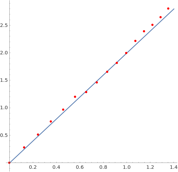
When the extension is over a prime field of modest size we can use methods that are efficient in practice.

Create a 12×12 random matrix over the integers modulo 7919, making the first two diagonal two elements into separate algebraic extension generators:

In[25]:=

Create dense generating polynomials and time the matrix minimal polynomial computation for extensions of increasing degrees:

In[26]:=

Out[27]=

A plot of the logarithms compared to a line with slope 2 shows what appears to be a quadratic relation between the timing of the matrix minimal polynomial computation and the size of the extension (as measured by the dimension of the vector space it generates over the base field):

In[28]:=

Out[28]=

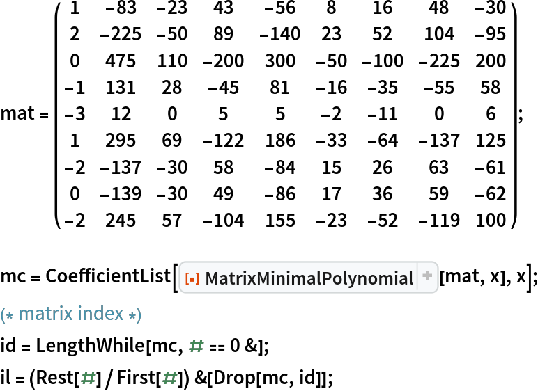
Neat Examples (3) 

Use MatrixMinimalPolynomial to compute the Drazin inverse of a singular matrix:

In[29]:=

Out[29]=

Verify some properties of the Drazin inverse:

In[30]:=

Out[30]=

In[31]:=

Out[31]=

Compare with the result of DrazinInverse:

In[32]:=

Out[32]=