Details
Moran's I can be computed by
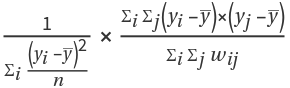
, where
wij is the value at position
(i,j) in
w (the weights matrix),
n is the length of the values list,

is the mean of the values list and
yi is the
ith element of the values list.
Moran's
I can also be computed using
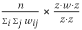
, where
n and
w are identical to the previous definition and
z is equal to
y-Mean[y].
values can be any (1D) list of real numbers, each of which are values of a different region, such as rainfall, area or elevation.
In Moranl[values,weights], weights must be a square matrix with length equal to the length of values and zeroes on the top-left–bottom-right diagonal, whose values represent the distance between the regions.
ResourceFunction["MoranI"] returns a real value n between -1 and 1, as follows:
| n = 1 | perfect correlation (values with a nonzero weight have identical values) |
| n ≈ 0 | no correlation with the weight matrix used (usually corresponding to random data, an improper weights matrix or no correlation) |
| n=-1 | perfect anticorrelation (values which have a nonzero weight have exactly opposite values) |
Often, although not always, weights is symmetrical along this diagonal, since the distance function used in its computation is usually commutative.
Moran's I is primarily used for geography/GIS, but can be applied in other fields.
ResourceFunction["MoranI"] can be used for data in any number of dimensions, since the input is only the values and distances, but multivariate autocorrelation is not supported.
When weights is not provided, the weights matrix is predefined such that the weights value at location (x,y) in the table is 1 if x and y are "next to" each other in values, and 0 otherwise.
There is no good way to select a weights matrix without knowing the source and shape of the data, but as long as the values are in a resonable order, the default weights matrix should provide somewhat meaningful results.
AutocorrelationTest and
ResourceFunction["MoranI"] both use a values list and calculate the correlation of that list with itself, but unlike
AutocorrelationTest, which uses either adjacent elements in the list or a lag of arbitrary length,
ResourceFunction["MoranI"] can be used with an arbitrary weights matrix to define the relations between elements.
Moran's
I allows for setting weight values other than 0 and 1 (especially useful if the weight of correlation is proportional to the distance), while
AutocorrelationTest assumes that elements exactly 1 "step" away (or exactly
n steps, if you are using a lag value) have a weight of 1 and everything else has a weight of 0.
Moran's I is very specific to an individual weight matrix, giving completely different results if the weights are changed. Due to this, values returned by ResourceFunction["MoranI"] cannot be compared with each other if the weights matrix is different, making it less useful for surveys across multiple regions.
ResourceFunction["MoranI"] supports symbolic computation.
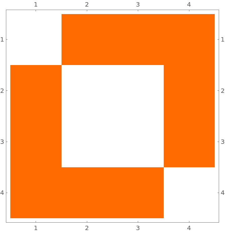
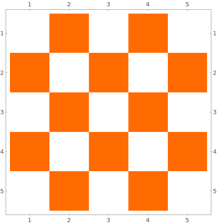


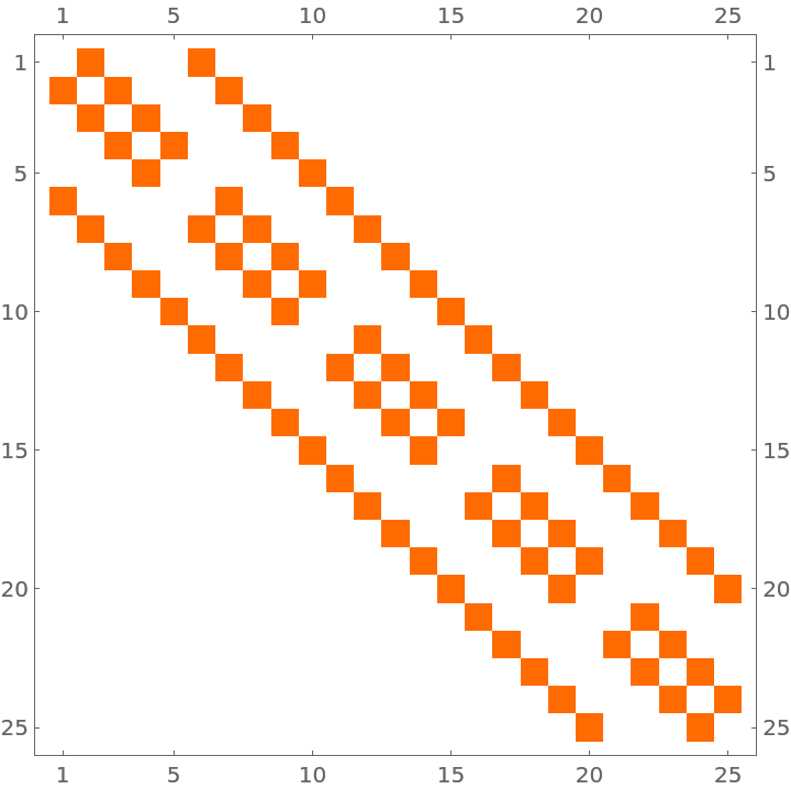
![weightTest1 = Sign@ReplacePart[
RegionMeasure[#, 1] & /@ Table[RegionIntersection[testReg1[[i]], testReg1[[j]]], {i, Length[testReg1]}, {j, Length[testReg1]}], Table[{i, i}, {i, Length[testReg1]}] -> 0]; MatrixPlot[weightTest1]](https://www.wolframcloud.com/obj/resourcesystem/images/c92/c9216ba8-2d08-449f-867a-bc54e2009a73/496dbabc9081c1c7.png)
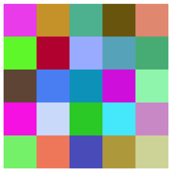
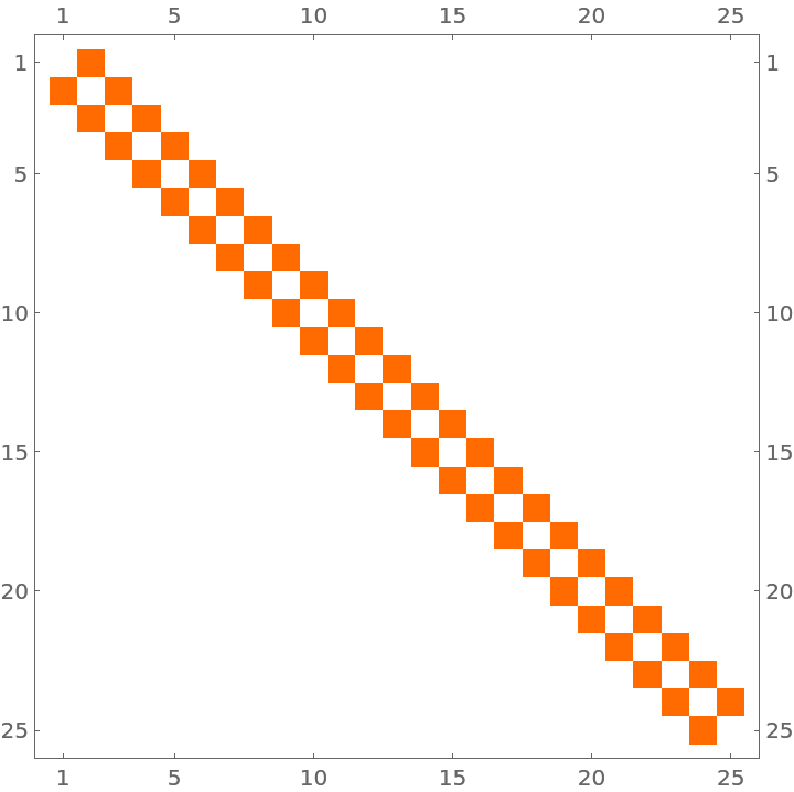
![testVals1 = Mod[Total /@ testReg1[[All, 1]], 2]; MatrixPlot[
Partition[testVals1, 5]]; ResourceFunction[
"MoranI"][testVals1, weightTest1]](https://www.wolframcloud.com/obj/resourcesystem/images/c92/c9216ba8-2d08-449f-867a-bc54e2009a73/21f26bebb6295da4.png)
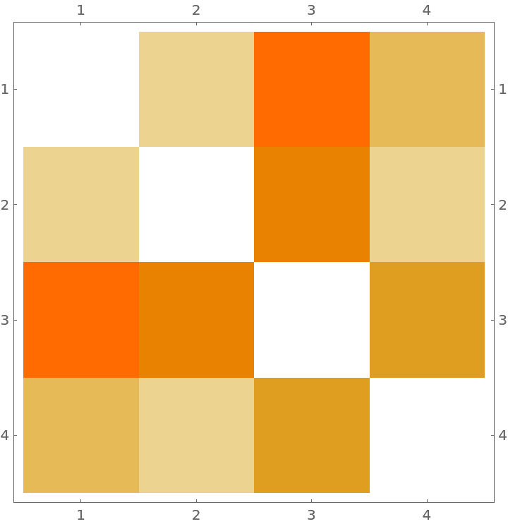
![saCountries = EntityList[EntityClass["Country", "SouthAmerica"]];
len = Length[saCountries];
borderlength = Table[If[i == j, 0, GeoLength@
GeoPath[GeoPosition /@ Flatten[border[saCountries[[i]], saCountries[[j]]], 1], "Geodesic"]], {i, 1, len}, {j, 1, len}];](https://www.wolframcloud.com/obj/resourcesystem/images/c92/c9216ba8-2d08-449f-867a-bc54e2009a73/59a5cf673c64d201.png)