Wolfram Function Repository
Instant-use add-on functions for the Wolfram Language
Function Repository Resource:
Compute the orthotomic of a curve
ResourceFunction["Orthotomic"][c,t] computes the orthotomic in parameter t of a curve c with respect to the point {0,0}. | |
ResourceFunction["Orthotomic"][c,p,t] computes the orthotomic with respect to the point p. | |
ResourceFunction["Orthotomic"][c,l,t] computes the orthotomic with respect to the infinite line l. |
Orthotomic of a circle with respect to the origin:
| In[1]:= |
| Out[1]= |
| In[2]:= |
| Out[2]= | 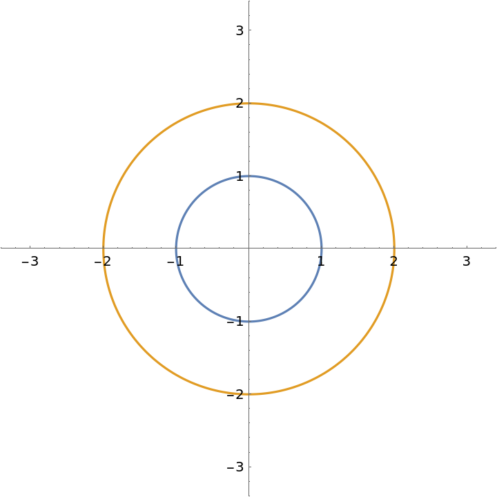 |
Orthotomic of a circle with respect to the point {1,1}:
| In[3]:= |
| Out[3]= |
| In[4]:= |
| Out[4]= | 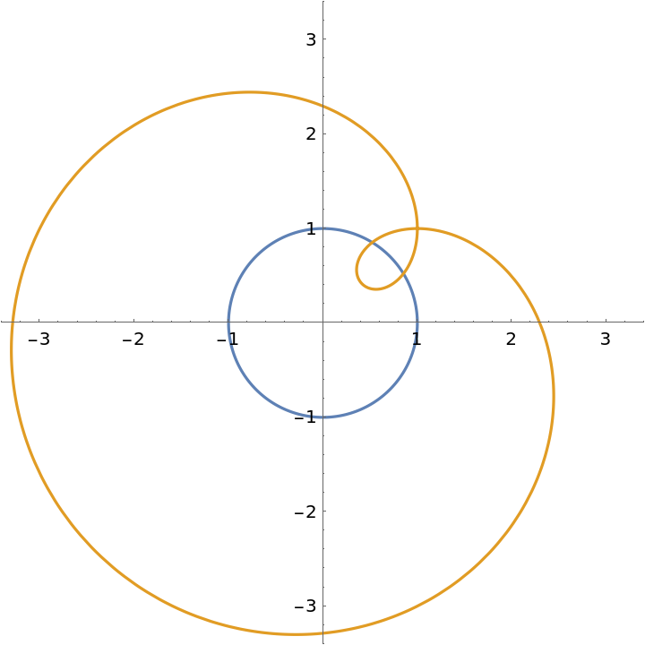 |
Orthotomic of an eight curve with respect to a varying point:
| In[5]:= |
| In[6]:= | ![Manipulate[
ParametricPlot[
Evaluate[{eight[t], ResourceFunction["Orthotomic"][eight[t], p, t]}], {t, 0, 2 \[Pi]},
PlotRange -> 3.4], {{p, {0, 0}}, Locator}, SaveDefinitions -> True]](https://www.wolframcloud.com/obj/resourcesystem/images/b9f/b9fe14e9-5046-4e81-9f27-aebf5f5d7976/701892b55583b20a.png) |
| Out[6]= | 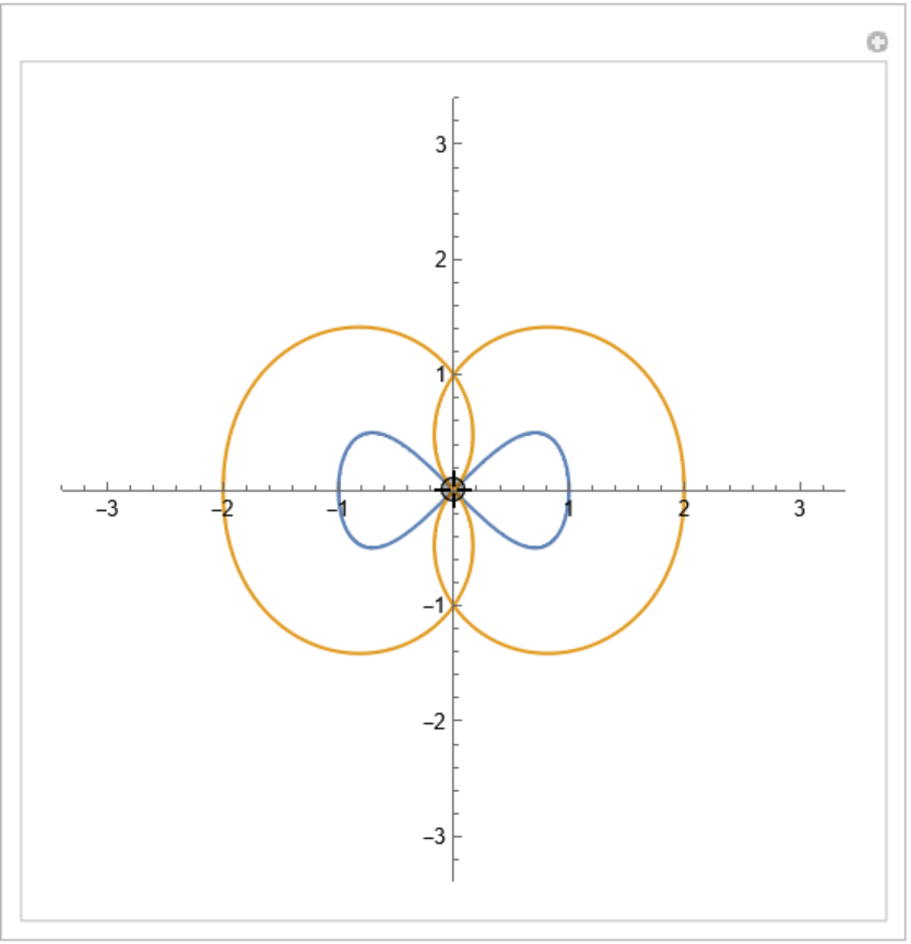 |
Parametric equations for a deltoid:
| In[7]:= |
| Out[7]= |
Orthotomic of the deltoid with respect to a given line:
| In[8]:= |
| Out[8]= |
| In[9]:= |
| Out[9]= | 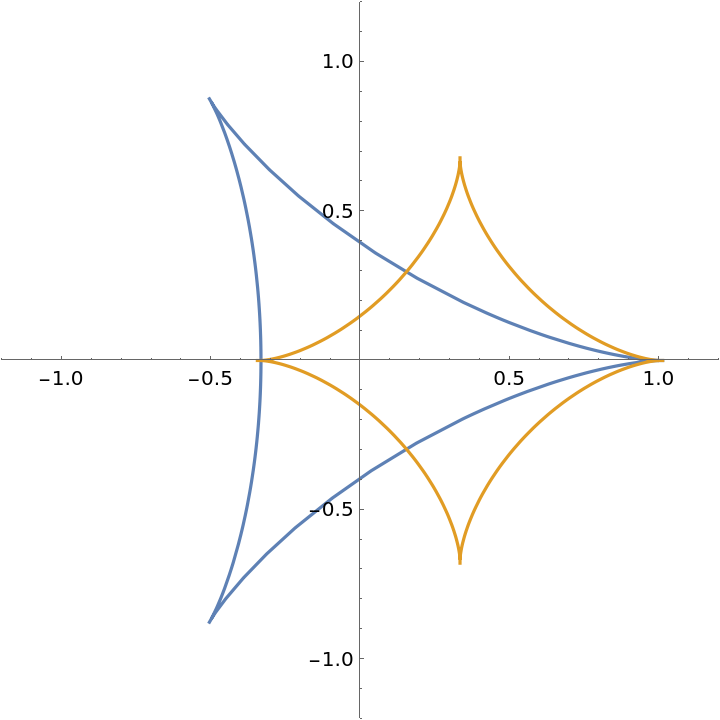 |
Orthotomic of a bifolium with respect to a varying line:
| In[10]:= |
| In[11]:= | ![Manipulate[
ParametricPlot[
Evaluate[{bifolium[t], ResourceFunction["Orthotomic"][eight[t], InfiniteLine[{p1, p2}], t]}], {t, 0, 2 \[Pi]}, Prolog -> {Directive[DotDashed, Gray, Thickness[Medium]], InfiniteLine[{p1, p2}]}, PlotRange -> 3.4], {{p1, {0, 0}}, Locator}, {{p2, {1, 1}}, Locator}, SaveDefinitions -> True]](https://www.wolframcloud.com/obj/resourcesystem/images/b9f/b9fe14e9-5046-4e81-9f27-aebf5f5d7976/0cf0aa259b0f02dd.png) |
| Out[11]= |  |
The orthotomic is equivalent to the pedal curve, scaled by a factor of 2:
| In[12]:= |
| In[13]:= |
| Out[13]= |
| In[14]:= |
| Out[14]= |
| In[15]:= |
| Out[15]= |
| In[16]:= |
| Out[16]= | 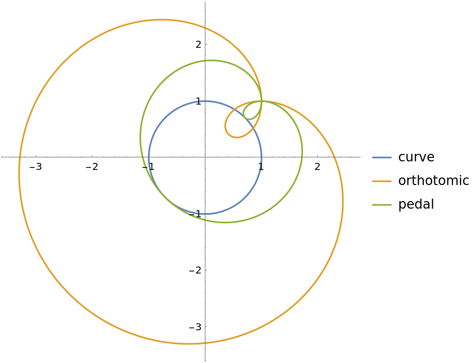 |
The catacaustic curve is the evolute of the orthotomic:
| In[17]:= |
| In[18]:= |
| Out[18]= |
| In[19]:= |
| Out[19]= |
| In[20]:= |
| Out[20]= |
| In[21]:= |
| Out[21]= | 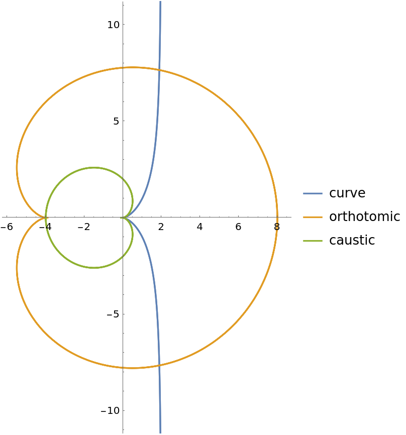 |
Generate the orthotomic as an envelope of circles:
| In[22]:= |
| In[23]:= |
| Out[23]= |
| In[24]:= | ![ParametricPlot[{curve[t], ot} // Evaluate, {t, -\[Pi], \[Pi]}, Prolog -> {Directive[Opacity[0.6, Gray], DotDashed], Table[N@Circle[curve[t], Norm[pt - curve[t]]], {t, -\[Pi] + \[Pi]/31, \[Pi] - \[Pi]/
31, \[Pi]/31}]}, PlotLegends -> {"curve", "orthotomic"}, PlotRange -> 2.9]](https://www.wolframcloud.com/obj/resourcesystem/images/b9f/b9fe14e9-5046-4e81-9f27-aebf5f5d7976/02d1075e14d49b85.png) |
| Out[24]= | 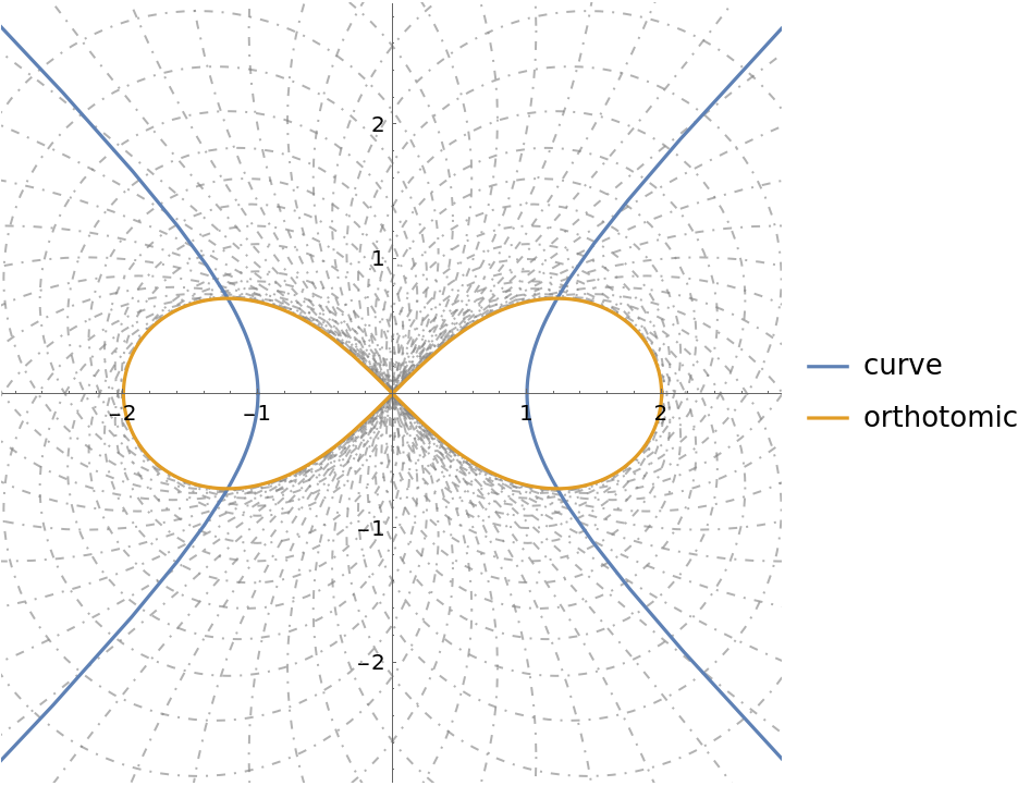 |
This work is licensed under a Creative Commons Attribution 4.0 International License