Wolfram Function Repository
Instant-use add-on functions for the Wolfram Language
Function Repository Resource:
Compute the orthotomic of a curve
ResourceFunction["Orthotomic"][c,t] computes the orthotomic in parameter t of a curve c with respect to the point {0,0}. | |
ResourceFunction["Orthotomic"][c,p,t] computes the orthotomic with respect to the point p. |
Orthotomic of a circle with respect to the point {1,1}:
| In[1]:= |
| Out[1]= |
| In[2]:= |
| Out[2]= | 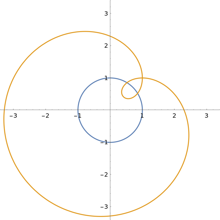 |
Orthotomic of a figure eight:
| In[3]:= |
| In[4]:= | ![Manipulate[
ParametricPlot[
Evaluate[{eight[t], ResourceFunction["Orthotomic"][eight[t], p, t]}], {t, 0, 2 \[Pi]},
PlotRange -> 3.4], {{p, {0, 0}}, {-\[Pi], -\[Pi]}, {\[Pi], \[Pi]}}]](https://www.wolframcloud.com/obj/resourcesystem/images/b9f/b9fe14e9-5046-4e81-9f27-aebf5f5d7976/1-0-0/523f242c3f306366.png) |
| Out[4]= | 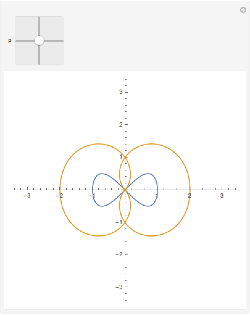 |
Pedal curves look similar to the orthotomic:
| In[5]:= |
| Out[5]= |
| In[6]:= | ![ParametricPlot[
Evaluate[{{Cos[t], Sin[t]}, ResourceFunction["Orthotomic"][{Cos[t], Sin[t]}, {1, 1}, t], pc}], {t, 0, 2 \[Pi]}, PlotRange -> 3.4]](https://www.wolframcloud.com/obj/resourcesystem/images/b9f/b9fe14e9-5046-4e81-9f27-aebf5f5d7976/1-0-0/5e23e80e57ffb5c8.png) |
| Out[6]= | 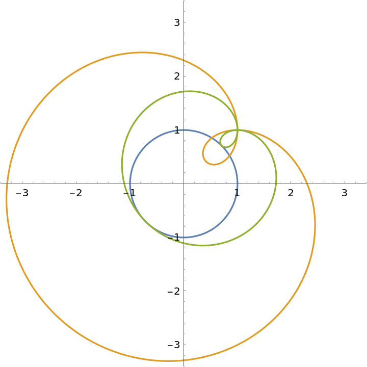 |
This work is licensed under a Creative Commons Attribution 4.0 International License