Wolfram Function Repository
Instant-use add-on functions for the Wolfram Language
Function Repository Resource:
Simulate hard spheres moving in an n-dimensional box
ResourceFunction["HardSphereSimulation"][assoc] generates a simulation of the motion of a system of hard spheres with simulation parameters specified by assoc. |
| "Positions" | initial particle positions |
| "Velocities" | initial particle velocities |
| "BoxSize" | side-length of simulation box |
| "Steps" | number of simulation time steps |
| "StepSize" | duration of a single time step |
| "BoundaryCondition" | interaction between particles and container walls |
| "Output" | simulation output |
| "ParticleRadius" | radius of spheres |
| "ParticleMass" | mass of spheres |
| "Reflecting" | particle velocities reflect upon contact with container walls |
| "Periodic" | particles are translated to opposite side of box upon reaching container walls |
| "Infinite" | particles do not alter motion upon reaching container walls |
| "PositionsByTime" | list of all particle positions at every time step |
| "VelocitiesByTime" | list of all particle velocities at every time step |
| "SpeedsByTime" | list of all particle speeds at every time step |
| "TrajectoriesByTime" | list of all particle positions and velocities at every time step |
| "PositionsByParticle" | list of positions over time for each particle |
| "VelocitiesByParticle" | list of velocities over time for each particle |
| "SpeedsByParticle" | list of speeds over time for each particle |
| "TrajectoriesByParticle" | list of positions and velocities over time for each particle |
| "Collisions" | list of particle-particle collisions |
| "All" | list containing “TrajectoriesByTime” output as the first entry, and “Collisions” as the second |
| "Visualize" | Graphics object with a Manipulate slider for visualizing the time-evolution of the system in one, two, or three spatial dimensions |
| "KineticEnergy" | list of total kinetic energy at every time step |
| "Temperature" | list of temperature at every time step |
| "CausalGraph" | Graph object with nodes representing collisions and directed edges indicating that one particle was contiguously involved in two collisions |
Simulate the motion of two hard disks over five time steps, and extract the trajectory data in various ways. Get the positions over time:
| In[1]:= | ![ResourceFunction[
"HardSphereSimulation"][<|"Positions" -> {{-2, -2}, {2, 2}}, "Velocities" -> {{1, 0}, {-1, 0}}, "BoxSize" -> 10, "ParticleRadius" -> 1, "Steps" -> 5, "StepSize" -> 1, "BoundaryCondition" -> "Reflecting",
"Output" -> "PositionsByTime"|>]](https://www.wolframcloud.com/obj/resourcesystem/images/aad/aadbf909-b609-4fcc-bd0b-3bcf350f8950/6d62df2c1e0b3264.png) |
| Out[1]= |
Get the velocities over time:
| In[2]:= | ![ResourceFunction[
"HardSphereSimulation"][<|"Positions" -> {{-2, -2}, {2, 2}}, "Velocities" -> {{1, 0}, {-1, 0}}, "BoxSize" -> 10, "ParticleRadius" -> 1, "Steps" -> 5, "StepSize" -> 1, "BoundaryCondition" -> "Reflecting",
"Output" -> "VelocitiesByTime"|>]](https://www.wolframcloud.com/obj/resourcesystem/images/aad/aadbf909-b609-4fcc-bd0b-3bcf350f8950/519617ef1f2b5d36.png) |
| Out[2]= |
Get the speeds over time:
| In[3]:= | ![ResourceFunction[
"HardSphereSimulation"][<|"Positions" -> {{-2, -2}, {2, 2}}, "Velocities" -> {{1, 0}, {-1, 0}}, "BoxSize" -> 10, "ParticleRadius" -> 1, "Steps" -> 5, "StepSize" -> 1, "BoundaryCondition" -> "Reflecting",
"Output" -> "SpeedsByTime"|>]](https://www.wolframcloud.com/obj/resourcesystem/images/aad/aadbf909-b609-4fcc-bd0b-3bcf350f8950/2254ba6fdbeef0ea.png) |
| Out[3]= |
Get the trajectories over time:
| In[4]:= | ![ResourceFunction[
"HardSphereSimulation"][<|"Positions" -> {{-2, -2}, {2, 2}}, "Velocities" -> {{1, 0}, {-1, 0}}, "BoxSize" -> 10, "ParticleRadius" -> 1, "Steps" -> 5, "StepSize" -> 1, "BoundaryCondition" -> "Reflecting",
"Output" -> "TrajectoriesByTime"|>]](https://www.wolframcloud.com/obj/resourcesystem/images/aad/aadbf909-b609-4fcc-bd0b-3bcf350f8950/1e07c96e6506b2e4.png) |
| Out[4]= |
Get the positions grouped by particle:
| In[5]:= | ![ResourceFunction[
"HardSphereSimulation"][<|"Positions" -> {{-2, -2}, {2, 2}}, "Velocities" -> {{1, 0}, {-1, 0}}, "BoxSize" -> 10, "ParticleRadius" -> 1, "Steps" -> 5, "StepSize" -> 1, "BoundaryCondition" -> "Reflecting",
"Output" -> "PositionsByParticle"|>]](https://www.wolframcloud.com/obj/resourcesystem/images/aad/aadbf909-b609-4fcc-bd0b-3bcf350f8950/0b10e9e6be2d0bb1.png) |
| Out[5]= |
Get the velocities grouped by particle:
| In[6]:= | ![ResourceFunction[
"HardSphereSimulation"][<|"Positions" -> {{-2, -2}, {2, 2}}, "Velocities" -> {{1, 0}, {-1, 0}}, "BoxSize" -> 10, "ParticleRadius" -> 1, "Steps" -> 5, "StepSize" -> 1, "BoundaryCondition" -> "Reflecting",
"Output" -> "VelocitiesByParticle"|>]](https://www.wolframcloud.com/obj/resourcesystem/images/aad/aadbf909-b609-4fcc-bd0b-3bcf350f8950/713b940aa9dc31a3.png) |
| Out[6]= |
Get the speeds grouped by particle:
| In[7]:= | ![ResourceFunction[
"HardSphereSimulation"][<|"Positions" -> {{-2, -2}, {2, 2}}, "Velocities" -> {{1, 0}, {-1, 0}}, "BoxSize" -> 10, "ParticleRadius" -> 1, "Steps" -> 5, "StepSize" -> 1, "BoundaryCondition" -> "Reflecting",
"Output" -> "SpeedsByParticle"|>]](https://www.wolframcloud.com/obj/resourcesystem/images/aad/aadbf909-b609-4fcc-bd0b-3bcf350f8950/3281fb8dc0032c87.png) |
| Out[7]= |
Get the trajectories grouped by particle:
| In[8]:= | ![ResourceFunction[
"HardSphereSimulation"][<|"Positions" -> {{-2, -2}, {2, 2}}, "Velocities" -> {{1, 0}, {-1, 0}}, "BoxSize" -> 10, "ParticleRadius" -> 1, "Steps" -> 5, "StepSize" -> 1, "BoundaryCondition" -> "Reflecting",
"Output" -> "TrajectoriesByParticle"|>]](https://www.wolframcloud.com/obj/resourcesystem/images/aad/aadbf909-b609-4fcc-bd0b-3bcf350f8950/320a88877af5ca07.png) |
| Out[8]= |
Use trajectory data to visualize frames from a hard sphere simulation:
| In[9]:= | ![Module[{trajectory}, (*Compute trajectories*)
trajectory = ResourceFunction[
"HardSphereSimulation"][<|
"Positions" -> Catenate@Table[{-14 + 2.5 i, 14 - 2.5 j}, {i, 4}, {j, 4}], "Velocities" -> Table[.5 {1, -1}, 16], "BoxSize" -> 30, "StepSize" -> 0.1, "ParticleRadius" -> 1, "Steps" -> 2000, "BoundaryCondition" -> "Reflecting", "Output" -> "TrajectoriesByParticle"|>]; (*Display snapshots of disks with velocity vectors*)
GraphicsGrid[Partition[Table[
Graphics[{Style[Disk[#[[1]], 1], Orange], Arrow[{#[[1]], #[[1]] + 4 #[[2]]}]} & /@ trajectory[[All, t]],
PlotRange -> 15, Frame -> True, FrameTicks -> None, ImageSize -> 100], {t, 1, 2000, 100}], 5], Spacings -> {5, 5}]]](https://www.wolframcloud.com/obj/resourcesystem/images/aad/aadbf909-b609-4fcc-bd0b-3bcf350f8950/1453f320ccaa020e.png) |
| Out[9]= | 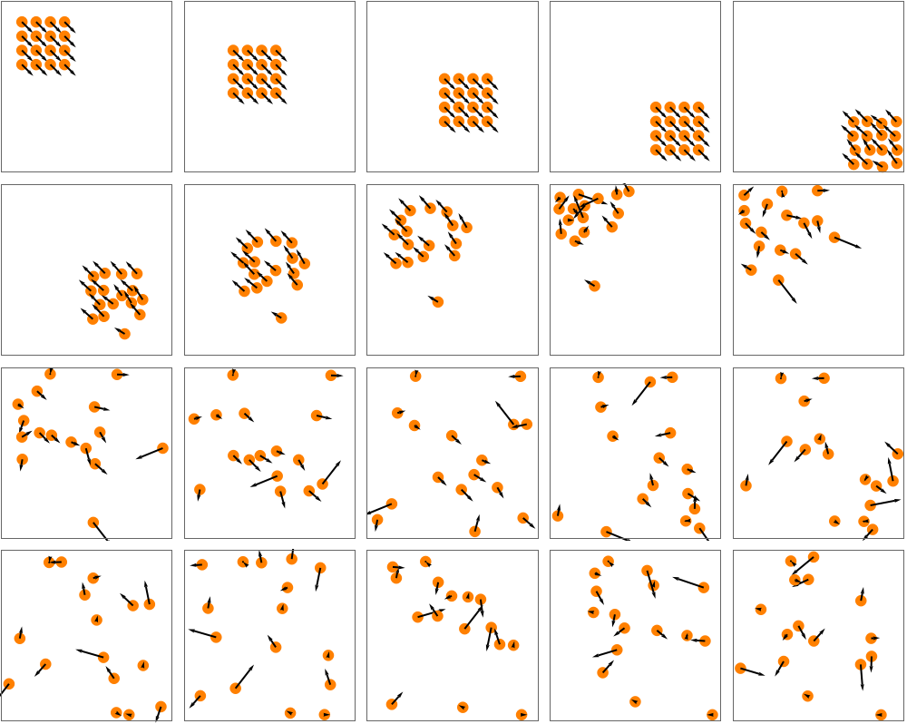 |
Use "Visualize" to generate an interactive visualization of many hard spheres moving in a box:
| In[10]:= | ![ResourceFunction[
"HardSphereSimulation"][<|"Positions" -> 3.2 N[CirclePoints[10]], "Velocities" -> N[CirclePoints[10]], "BoxSize" -> 20, "ParticleRadius" -> 1, "Steps" -> 200, "StepSize" -> 0.1, "BoundaryCondition" -> "Reflecting", "Output" -> "Visualize"|>]](https://www.wolframcloud.com/obj/resourcesystem/images/aad/aadbf909-b609-4fcc-bd0b-3bcf350f8950/1a6ed12d94b10487.png) |
| Out[10]= | 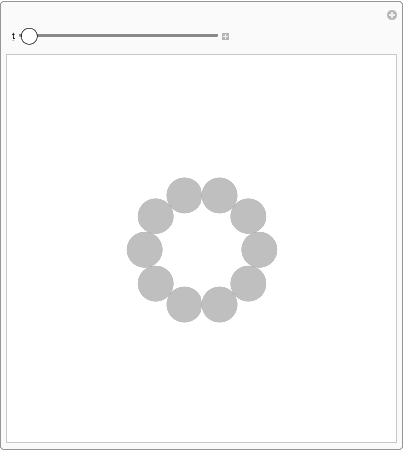 |
Use "RandomNonOverlapping" to generate random non-overlapping initial positions in the box:
| In[11]:= | ![ResourceFunction[
"HardSphereSimulation"][<|"Positions" -> "RandomNonOverlapping", "Velocities" -> RandomPoint[Ball[{0, 0}, 1], 15], "BoxSize" -> 10, "ParticleRadius" -> 1, "Steps" -> 200, "StepSize" -> 0.1, "BoundaryCondition" -> "Reflecting", "Output" -> "Visualize"|>]](https://www.wolframcloud.com/obj/resourcesystem/images/aad/aadbf909-b609-4fcc-bd0b-3bcf350f8950/7688a779f4f5f628.png) |
| Out[11]= | 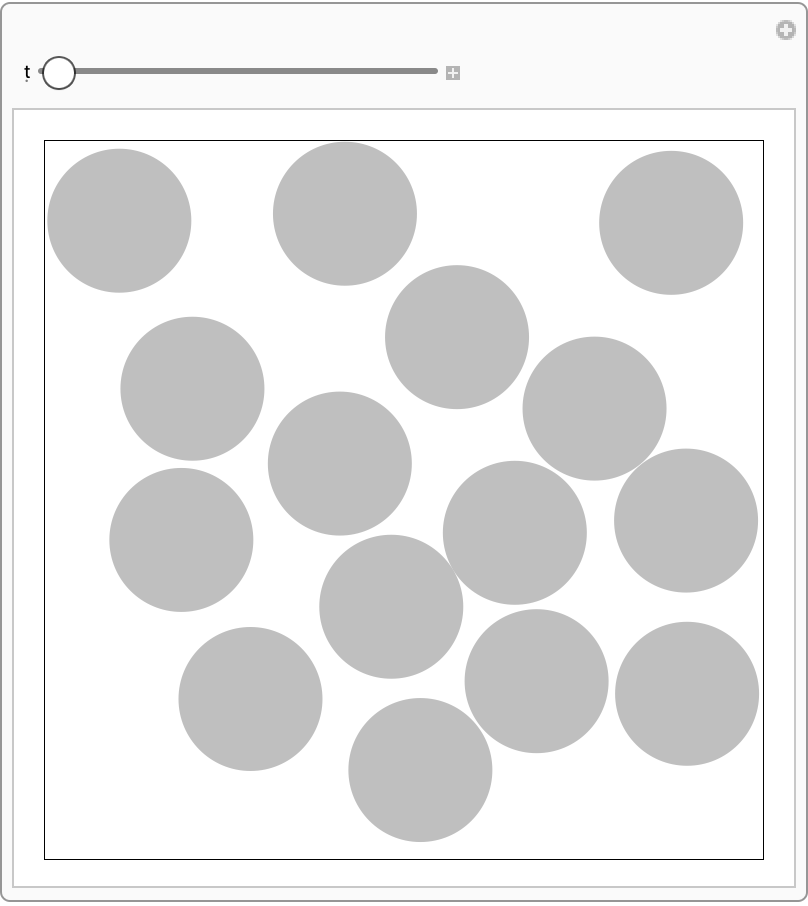 |
Visualization works in 1D:
| In[12]:= | ![ResourceFunction[
"HardSphereSimulation"][<|"Positions" -> "RandomNonOverlapping", "Velocities" -> RandomPoint[Ball[{0}, 1], 15], "BoxSize" -> 60, "ParticleRadius" -> 1, "Steps" -> 500, "StepSize" -> 0.1, "BoundaryCondition" -> "Reflecting", "Output" -> "Visualize"|>]](https://www.wolframcloud.com/obj/resourcesystem/images/aad/aadbf909-b609-4fcc-bd0b-3bcf350f8950/78a96663b3c39731.png) |
| Out[12]= | 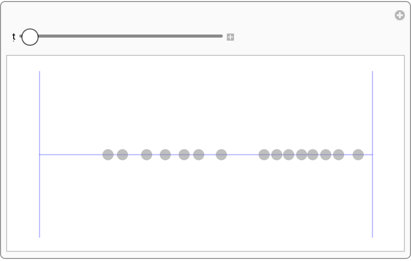 |
Visualization works in 3D as well:
| In[13]:= | ![ResourceFunction[
"HardSphereSimulation"][<|"Positions" -> "RandomNonOverlapping", "Velocities" -> RandomPoint[Ball[{0, 0, 0}, 1], 10], "BoxSize" -> 6,
"ParticleRadius" -> 1, "Steps" -> 500, "StepSize" -> 0.1, "BoundaryCondition" -> "Reflecting", "Output" -> "Visualize"|>]](https://www.wolframcloud.com/obj/resourcesystem/images/aad/aadbf909-b609-4fcc-bd0b-3bcf350f8950/532bc069ab303aa0.png) |
| Out[13]= | 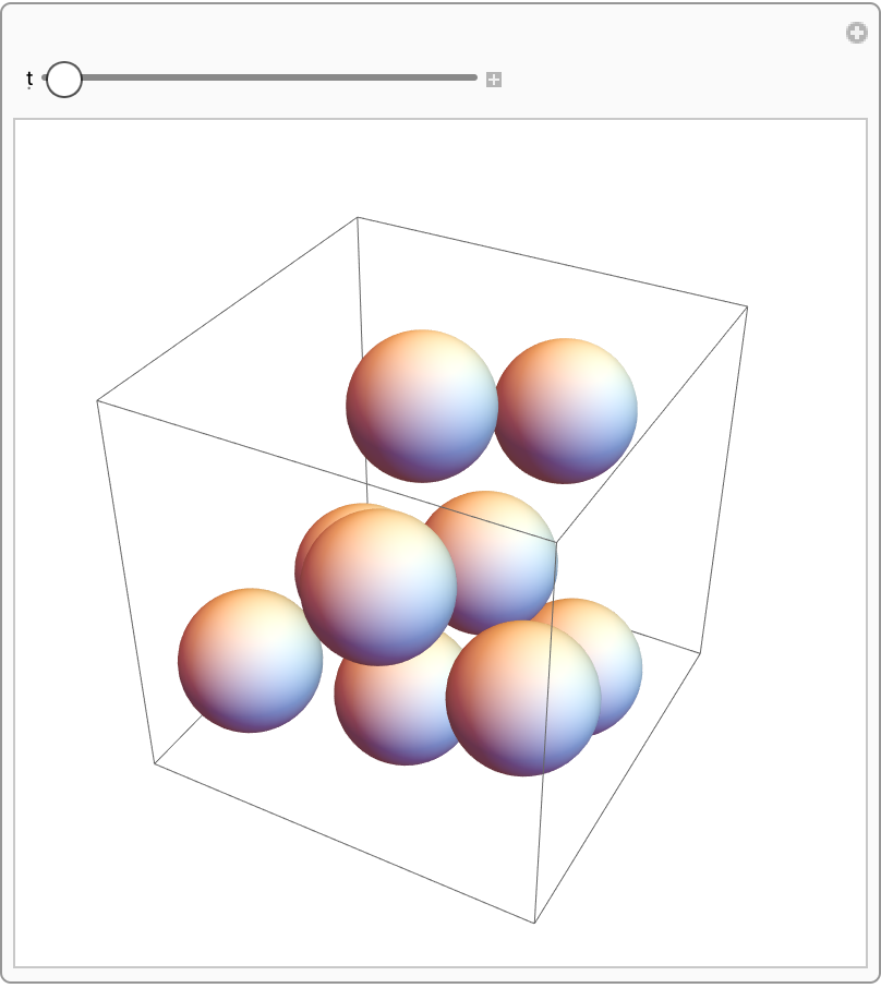 |
Periodic boundary conditions identify opposite walls of the box with one another:
| In[14]:= | ![ResourceFunction[
"HardSphereSimulation"][<|"Positions" -> "RandomNonOverlapping", "Velocities" -> RandomPoint[Ball[{0, 0}, 1], 15], "BoxSize" -> 10, "ParticleRadius" -> 1, "Steps" -> 500, "StepSize" -> 0.1, "BoundaryCondition" -> "Periodic", "Output" -> "Visualize"|>]](https://www.wolframcloud.com/obj/resourcesystem/images/aad/aadbf909-b609-4fcc-bd0b-3bcf350f8950/4775b4152bf30e72.png) |
| Out[14]= |  |
Infinite boundary conditions eliminate particle-wall interactions altogether:
| In[15]:= | ![ResourceFunction[
"HardSphereSimulation"][<|"Positions" -> "RandomNonOverlapping", "Velocities" -> RandomPoint[Ball[{0, 0}, 1], 15], "BoxSize" -> 10, "ParticleRadius" -> 1, "Steps" -> 300, "StepSize" -> 0.1, "BoundaryCondition" -> "Infinite", "Output" -> "Visualize"|>]](https://www.wolframcloud.com/obj/resourcesystem/images/aad/aadbf909-b609-4fcc-bd0b-3bcf350f8950/718878330f1b2391.png) |
| Out[15]= | 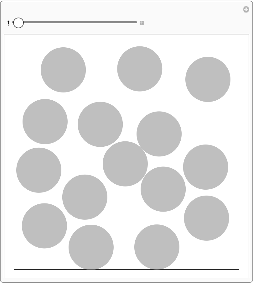 |
Multiple outputs can be returned at once:
| In[16]:= | ![ResourceFunction["HardSphereSimulation"][
<|"Positions" -> "RandomNonOverlapping",
"Velocities" -> RandomPoint[Ball[{0, 0}, 1], 15],
"BoxSize" -> 10, "ParticleRadius" -> 1, "Steps" -> 5, "StepSize" -> 0.1, "BoundaryCondition" -> "Reflecting", "Output" -> {"KineticEnergy", "Temperature"}|>]](https://www.wolframcloud.com/obj/resourcesystem/images/aad/aadbf909-b609-4fcc-bd0b-3bcf350f8950/35e68ee3f61df7fb.png) |
| Out[16]= |
Particle speeds should obey Maxwell-Boltzmann distribution:
| In[17]:= | ![Module[{speeds, Temp},
{speeds, Temp} = {Flatten[#[[1]]], First[#[[2]]]} &@
ResourceFunction["HardSphereSimulation"][
<|"Positions" -> "RandomNonOverlapping",
"Velocities" -> RandomPoint[Ball[{0, 0}, 1], 15],
"BoxSize" -> 10, "ParticleRadius" -> 1, "Steps" -> 5000, "StepSize" -> 0.1, "BoundaryCondition" -> "Reflecting", "Output" -> {"SpeedsByTime", "Temperature"}|>]; Show[
(*Empirical histogram of speeds*)
Histogram[speeds, {0.1`}, "PDF", Frame -> True, FrameLabel -> (Style[#1, Black, 14] &) /@ {"v", "\[Rho](v)"}, PlotLabel -> Style["Speed Distribution with Maxwell-Boltzmann Fit", Black, 15],
ImageSize -> 400], (*Plot of 2D Maxwell-Boltzmann distribution with best-
fit temperature.*)
Plot[1/Temp v E^(-(v^2/(2 Temp))), {v, 0, 2}]
]
]](https://www.wolframcloud.com/obj/resourcesystem/images/aad/aadbf909-b609-4fcc-bd0b-3bcf350f8950/25a76ead84e9d467.png) |
| Out[17]= | 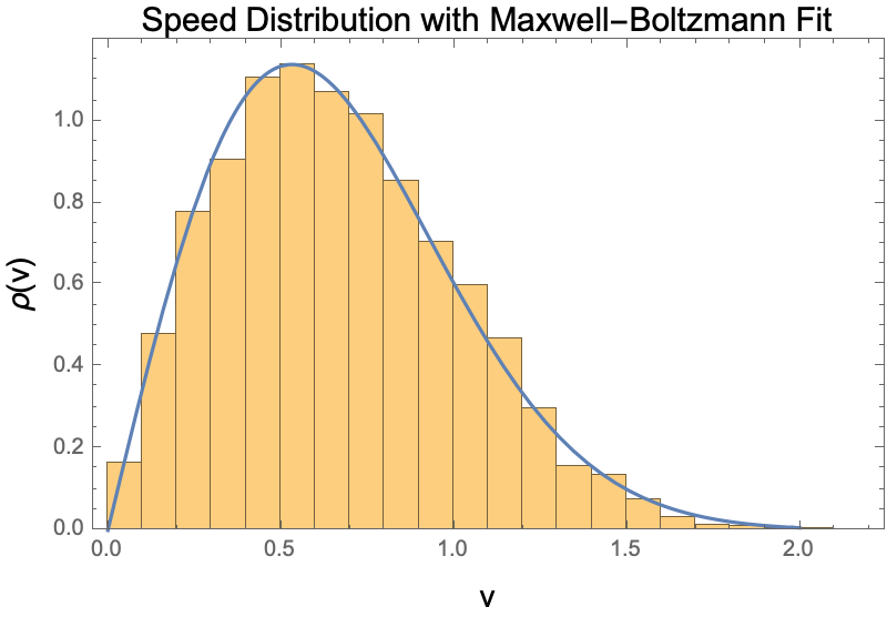 |
Extract a collision list from the simulation, where collisions take the form {particle1,particle2,time of collision}:
| In[18]:= | ![ResourceFunction["HardSphereSimulation"][
<|"Positions" -> {{-8, 0}, {-4, 0}, {0, 0}, {4, 0}, {8, 0}},
"Velocities" -> {{1, 0}, {0, 0}, {0, 0}, {0, 0}, {0, 0}},
"BoxSize" -> 20, "ParticleRadius" -> 1, "Steps" -> 200, "StepSize" -> 0.1, "BoundaryCondition" -> "Reflecting", "Output" -> "Collisions"|>]](https://www.wolframcloud.com/obj/resourcesystem/images/aad/aadbf909-b609-4fcc-bd0b-3bcf350f8950/4bb543373de149b6.png) |
| Out[18]= |
From particle-particle collisions, construct the causal graph:
| In[19]:= | ![ResourceFunction["HardSphereSimulation"][
<|"Positions" -> {{-8, 0}, {-4, 0}, {0, 0}, {4, 0}, {8, 0}},
"Velocities" -> {{1, 0}, {0, 0}, {0, 0}, {0, 0}, {0, 0}},
"BoxSize" -> 20, "ParticleRadius" -> 1, "Steps" -> 200, "StepSize" -> 0.1, "BoundaryCondition" -> "Reflecting", "Output" -> "CausalGraph"|>]](https://www.wolframcloud.com/obj/resourcesystem/images/aad/aadbf909-b609-4fcc-bd0b-3bcf350f8950/6db6b868dcef535b.png) |
| Out[19]= | 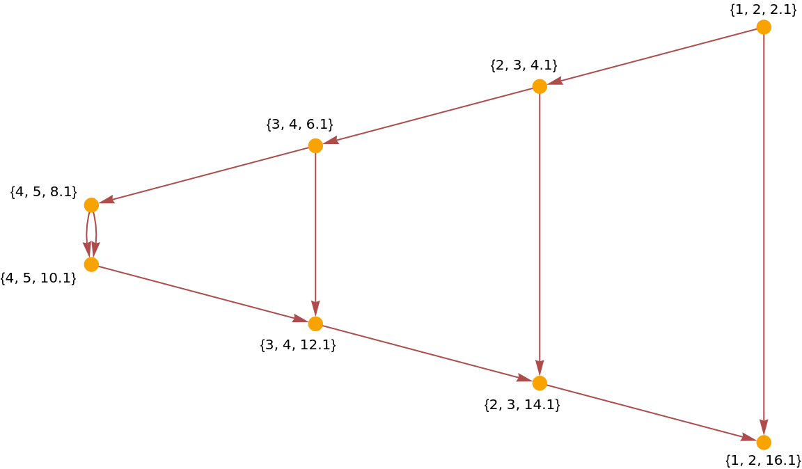 |
Construct a causal graph for a disordered system:
| In[20]:= | ![ResourceFunction["HardSphereSimulation"][
<|"Positions" -> "RandomNonOverlapping", "Velocities" -> RandomPoint[Ball[{0, 0}, 1], 15],
"BoxSize" -> 10, "ParticleRadius" -> 1, "Steps" -> 100, "StepSize" -> 0.1, "BoundaryCondition" -> "Reflecting", "Output" -> "CausalGraph"|>] // Graph[#, VertexLabels -> None] &](https://www.wolframcloud.com/obj/resourcesystem/images/aad/aadbf909-b609-4fcc-bd0b-3bcf350f8950/722b9f6d8a26989c.png) |
| Out[20]= | 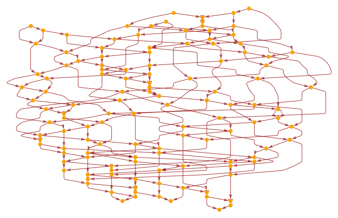 |
As the nodes of the causal graph represent collisions between two particles and the edges represent individual particles, we expect all nodes to have indegree and outdegree 2, besides from the graph boundary (i.e., the beginning and end of the simulation):
| In[21]:= |
| Out[21]= |
Total kinetic energy of spheres should be conserved in time. Show that the error stays within machine precision:
| In[22]:= | ![ListLinePlot[# - #[[1]] &[
ResourceFunction[
"HardSphereSimulation"][<|"Positions" -> "RandomNonOverlapping", "Velocities" -> RandomPoint[Ball[{0, 0}, 1], 15],
"BoxSize" -> 10, "ParticleRadius" -> 1, "Steps" -> 500, "StepSize" -> 0.1, "BoundaryCondition" -> "Reflecting", "Output" -> "KineticEnergy"|>]
], Frame -> True, FrameLabel -> {"Time Step", "E-\!\(\*SubscriptBox[\(E\), \(initial\)]\)"}, RotateLabel -> False, PlotLabel -> "Energy Conservation vs. Time", PlotRange -> {{0, 500}, Automatic}]](https://www.wolframcloud.com/obj/resourcesystem/images/aad/aadbf909-b609-4fcc-bd0b-3bcf350f8950/193cb25c07ef8003.png) |
| Out[22]= | 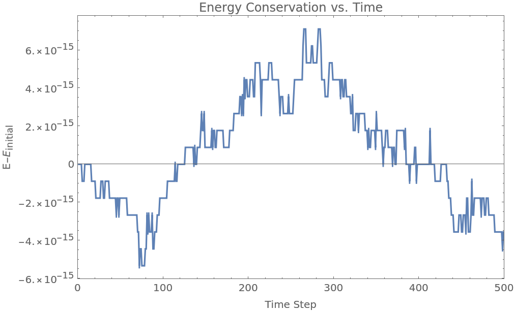 |
Momentum should be conserved during collisions between particles. Collision of equal mass particles:
| In[23]:= | ![ResourceFunction[
"HardSphereSimulation"][<|
"Positions" -> {{-8, 0}, {-4, 0}, {0, 0}, {4, 0}, {8, 0}},
"Velocities" -> {{1, 0}, {0, 0}, {0, 0}, {0, 0}, {0, 0}},
"BoxSize" -> 20, "ParticleRadius" -> 1, "ParticleMass" -> 2.0, "Steps" -> 200, "StepSize" -> 0.1, "BoundaryCondition" -> "Reflecting", "Output" -> "Visualize"|>]](https://www.wolframcloud.com/obj/resourcesystem/images/aad/aadbf909-b609-4fcc-bd0b-3bcf350f8950/4bf4f7c07e9defd4.png) |
| Out[23]= |  |
Collision of an incoming heavy particle with a much lighter stationary particle causes the light particle to go out with double the speed of the incoming one:
| In[24]:= | ![ResourceFunction[
"HardSphereSimulation"][<|
"Positions" -> {{-2.1, 0}, {0, 0}, {2.1, 0}},
"Velocities" -> {{1, 0}, {0, 0}, {0, 0}},
"BoxSize" -> 50, "ParticleRadius" -> 1, "Steps" -> 4, "StepSize" -> 0.1, "BoundaryCondition" -> "Reflecting", "Output" -> "SpeedsByTime", "ParticleMass" -> {10^10, 10^5, 1}|>]](https://www.wolframcloud.com/obj/resourcesystem/images/aad/aadbf909-b609-4fcc-bd0b-3bcf350f8950/1305c48e624b2d2c.png) |
| Out[24]= |
Collision of a very light particle with a much heavier stationary particle leads to reflection of the incoming particle:
| In[25]:= | ![ResourceFunction[
"HardSphereSimulation"][<|"Positions" -> {{0, 0}, {2.1, 0}},
"Velocities" -> {{1, 0}, {0, 0}},
"BoxSize" -> 20, "ParticleRadius" -> 1, "ParticleMass" -> {1, 10^5},
"Steps" -> 3, "StepSize" -> 0.1, "BoundaryCondition" -> "Reflecting", "Output" -> "VelocitiesByTime"|>]](https://www.wolframcloud.com/obj/resourcesystem/images/aad/aadbf909-b609-4fcc-bd0b-3bcf350f8950/5a6d03484bb72a45.png) |
| Out[25]= |
Particle overlaps are resolved pairwise, so situations involving multiple overlapping spheres may lead to unexpected results (such as a disruption of symmetry):
| In[26]:= | ![ResourceFunction[
"HardSphereSimulation"][<|"Positions" -> 3 N[CirclePoints[10]], "Velocities" -> N[CirclePoints[10]],
"BoxSize" -> 20, "ParticleRadius" -> 1, "Steps" -> 200, "StepSize" -> 0.1, "BoundaryCondition" -> "Reflecting", "Output" -> "Visualize"|>]](https://www.wolframcloud.com/obj/resourcesystem/images/aad/aadbf909-b609-4fcc-bd0b-3bcf350f8950/6a855e3251b78b7a.png) |
| Out[26]= | 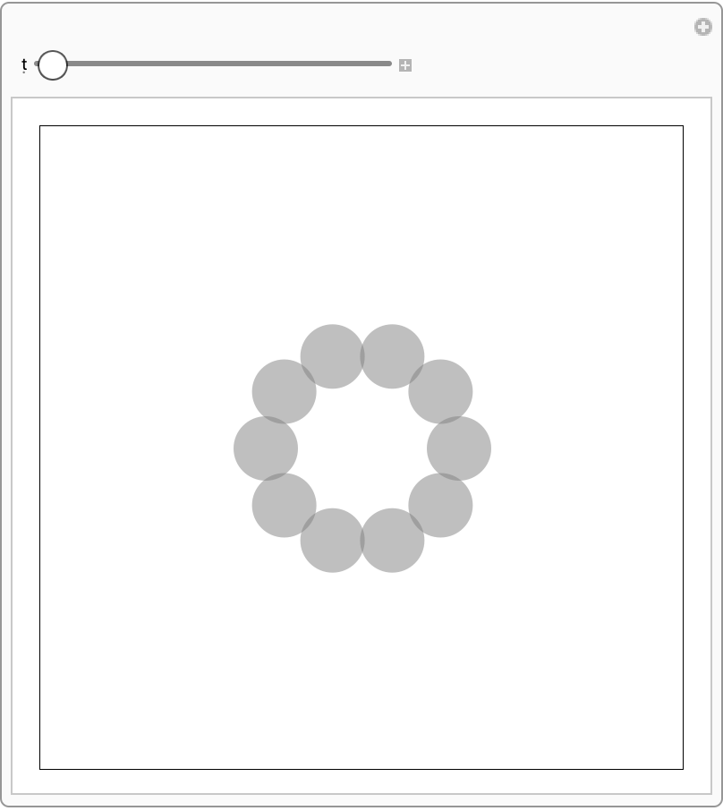 |
The "RandomNonOverlapping" option is not guaranteed to find non-overlapping configurations at very high packing fractions:
| In[27]:= | ![ResourceFunction[
"HardSphereSimulation"][<|"Positions" -> "RandomNonOverlapping", "Velocities" -> RandomPoint[Ball[{0, 0}], 25],
"BoxSize" -> 10, "ParticleRadius" -> 1, "Steps" -> 10, "StepSize" -> 0.1, "BoundaryCondition" -> "Reflecting", "Output" -> "Visualize"|>]](https://www.wolframcloud.com/obj/resourcesystem/images/aad/aadbf909-b609-4fcc-bd0b-3bcf350f8950/6bb372a5e04825dd.png) |
| Out[27]= | 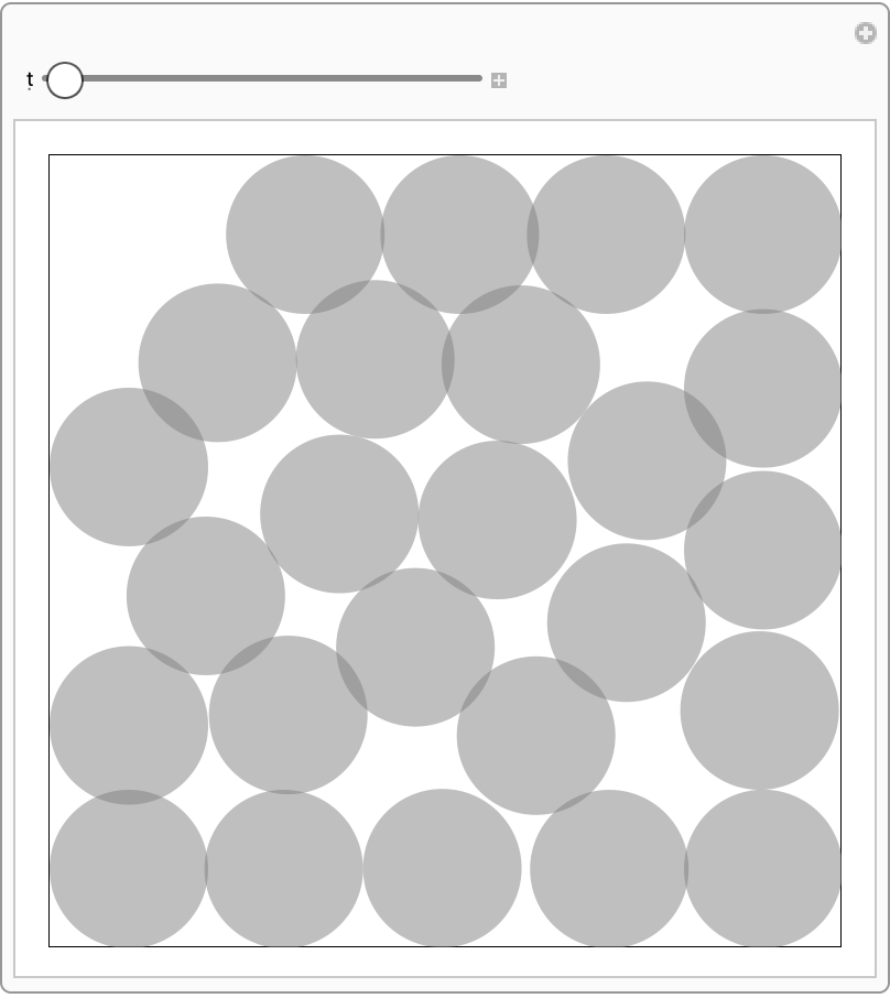 |
Simulate a Newton's cradle:
| In[28]:= | ![ResourceFunction["HardSphereSimulation"][<|
"Positions" -> {{-12, 0}, {-10, 0}, {-8, 0}, {-6, 0}, {-4, 0}, {-2, 0}, {0, 0}, {2, 0}, {4, 0}, {6, 0}, {8, 0}, {10, 0}, {12, 0}}, "Velocities" -> {{1, 0}, {0, 0}, {0, 0}, {0, 0}, {0, 0}, {0, 0}, {0,
0}, {0, 0}, {0, 0}, {0, 0}, {0, 0}, {0, 0}, {0, 0}},
"BoxSize" -> 40, "ParticleRadius" -> 1, "Steps" -> 500, "StepSize" -> 0.1, "BoundaryCondition" -> "Reflecting", "Output" -> "Visualize"|>]](https://www.wolframcloud.com/obj/resourcesystem/images/aad/aadbf909-b609-4fcc-bd0b-3bcf350f8950/462d2fce46ba9923.png) |
| Out[28]= | 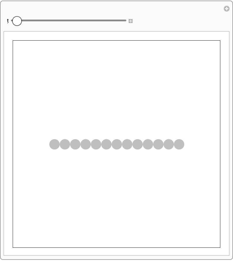 |
Use HardSphereSimulation to simulate a simplified game of pool:
| In[29]:= | ![(* Evaluate this cell to get the example input *) CloudGet["https://www.wolframcloud.com/obj/bcbf73c0-01b4-4e97-8f94-1fac2c153f4e"]](https://www.wolframcloud.com/obj/resourcesystem/images/aad/aadbf909-b609-4fcc-bd0b-3bcf350f8950/151bbae42971b165.png) |
| Out[32]= | 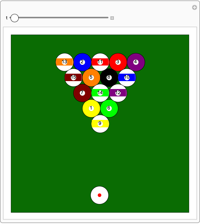 |
This work is licensed under a Creative Commons Attribution 4.0 International License