Function Repository Resource:

HardSphereSimulation (1.0.0) current version: 2.1.0 »

Simulate hard spheres moving in an N-dimensional box with reflecting boundary conditions

Contributed by: Matt Kafker and Christopher Wolfram

ResourceFunction["HardSphereSimulation"][pos,vel,boxsize,stepsize,rad,steps]

simulates a hard sphere gas comprised of identical particles of radius rad in a cube of side length 2boxsize, starting at the initial positions pos and corresponding initial velocities vel, for the given number of steps with each particle moving at stepsize times its velocity.

Details

ResourceFunction["HardSphereSimulation"] returns a list of the full state of the system at each time-step, and also a list of all collisions that occur during evolution.

The output has the form {{{p₁,v₁},{p₂,v₂},…},collisions}, where the p_i are the positions and the v_i are velocities and time i.

Each collision takes the form {particle_i,particle_j,stepofcollision}.

The dimensions of vectors in pos and vel determine the spatial dimension of system (they can be any positive integer dimension).

The box is centered on the origin, and boxsize refers to half of the side length of a square.

Examples

Basic Examples (2)

Simulate five steps of a single circular particle starting at the origin with velocity {4.0,0.2}:

In[1]:=

Out[1]=

Plot the position at each time:

In[2]:=

Out[2]=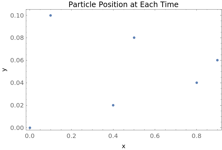

Scope (3)

Use HardSphereSimulation to visualize the evolution of a single hard sphere in a box:

In[3]:=

With[
(*Set parameters and initial conditions*)
{boxRadius = 5, ballRadius = 1, stepSize = 0.1, numSteps = 100, initialPosition = {1, 0}, initialVelocity = {-2, 5}}, (*Simulate one hard sphere in box*)
simulation = ResourceFunction[
"HardSphereSimulation"][{initialPosition}, {initialVelocity}, boxRadius, stepSize, ballRadius, numSteps]; (*Display result graphically*)
Manipulate[
Graphics[Disk[#, ballRadius] &@simulation[[1, All, 1, 1]][[t]], Sequence[
AspectRatio -> 1, PlotRange -> {{-5, 5}, {-5, 5}}, Frame -> True]], {t, 1, numSteps, 1}]
]

Out[3]=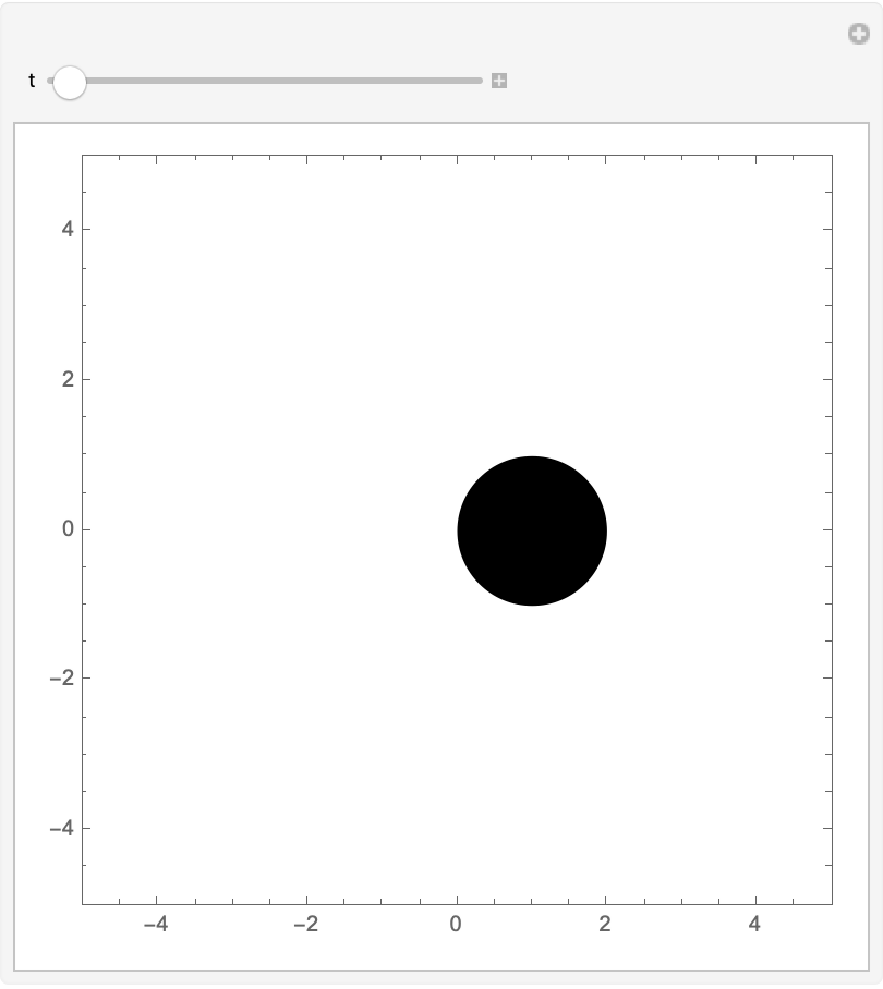

Use HardSphereSimulation to visualize many hard spheres moving in a box:

In[4]:=

$(*Define parameters for a model*) num = 50; steps = 200; boxSize = 15; rad = 1; stepSize = 0.1; (*Start with random initial conditions:*) initialPos = RandomReal[{-#, #} &@(boxSize - rad), {num, 2}]; initialVel = RandomPoint[Ball[ConstantArray[0, 2]], num]; (*Run simulation:*) traj = ResourceFunction["HardSphereSimulation"][initialPos, initialVel, boxSize, stepSize, rad, steps][[1, All, 1]]\[Transpose]; (*Visualize the results:*) Manipulate[ Graphics[{{ FaceForm[], EdgeForm[Black], Rectangle[{-boxSize, -boxSize}, {boxSize, boxSize}]}, Disk[#, rad] & /@ traj[[All, t]]}], {t, 1, Length[traj[[1]]], 1}]$

Out[8]=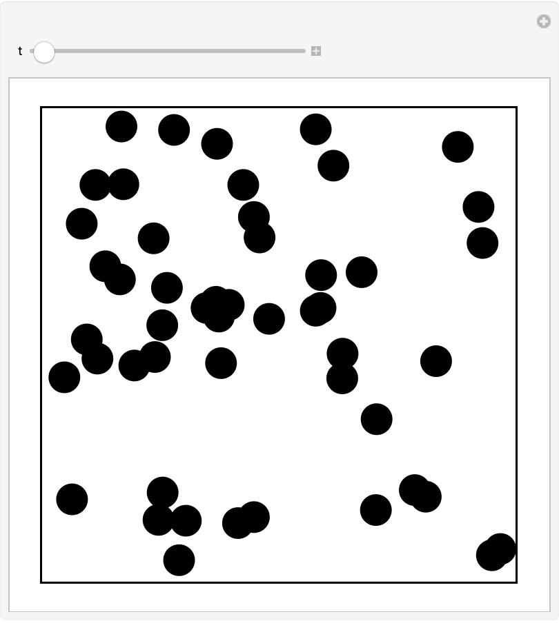

Derive causal graph from list of collisions:

In[9]:=

$(*Function to generate a causal graph from the collisions list.*) collisionsToCausalGraph[collisions_] := Module[{particles, instants, edges}, (*Extract particles from list of collisions*) particles = Union @@ collisions[[All, ;; 2]]; (*Generate causal graph from collisions. Construct a directed edge whenever an uninterrupted sequence of two collisions involves the same particle.*) edges = Catenate[Function[particle, instants = SplitBy[Select[ collisions, #[[1]] === particle || #[[2]] === particle &], Last]; Catenate[ BlockMap[DirectedEdge @@@ Tuples[#] &, instants, 2, 1]] ] /@ particles]; (*Finally, construct the graph*) Graph[DeleteDuplicates@edges, Sequence[ GraphLayout -> "LayeredDigraphEmbedding", AspectRatio -> 1/GoldenRatio, ImageSize -> Large]] ]$

In[10]:=

(*Run a simulation and extract the causal graph*)
With[{num = 15, steps = 50, boxSize = 5, dimension = 2, rad = 1, stepSize = 0.1}, Module[{collisions, initialPos, initialVel}, (*Random initial conditions*)
initialPos = RandomReal[{-#, #} &@(boxSize - rad), {num, dimension}];
initialVel = RandomPoint[Ball[ConstantArray[0, dimension]], num]; (*Run a simulation. Ignore first 20% to eliminate transient role of initial conditions.*)
collisions = Select[ResourceFunction["HardSphereSimulation"][
initialPos, initialVel, Sequence[
N[boxSize],
N[stepSize],
N[rad], steps]][[2]], #[[3]] > Round[steps/5] &]; (*Generate causal graph*)
collisionsToCausalGraph[collisions]
]
]

Out[10]=

Properties and Relations (1)

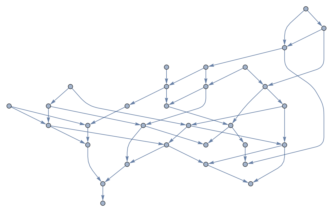Total kinetic energy of spheres should be conserved in time:

In[11]:=

$KE[sim_] := ListLinePlot[Total /@ Map[Norm[#]^2/2 &, sim[[All, 2]], {2}], Sequence[ PlotLabel -> Style["Kinetic Energy v. Simulation Step", 15, Black], Frame -> True, FrameLabel -> {"Simulation Step", "Kinetic Energy"}, PlotTheme -> "Scientific", ImageSize -> Medium]]$

In[12]:=

With[{num = 12, steps = 125, boxSize = 5, rad = 1, stepSize = 0.1, dimension = 5},
Module[{ initialPos, initialVel},
(*Randomly distributed initial positions and velocities*)
initialPos = N[RandomReal[{-#, #} &@boxSize, {num, dimension}]];
initialVel = N[RandomPoint[Ball[ConstantArray[0, dimension]], num]];
KE[ResourceFunction["HardSphereSimulation"][initialPos, initialVel, Sequence[
N[boxSize],
N[stepSize],
N[rad]], steps][[1]]]]]

Out[12]=

Neat Examples (1)

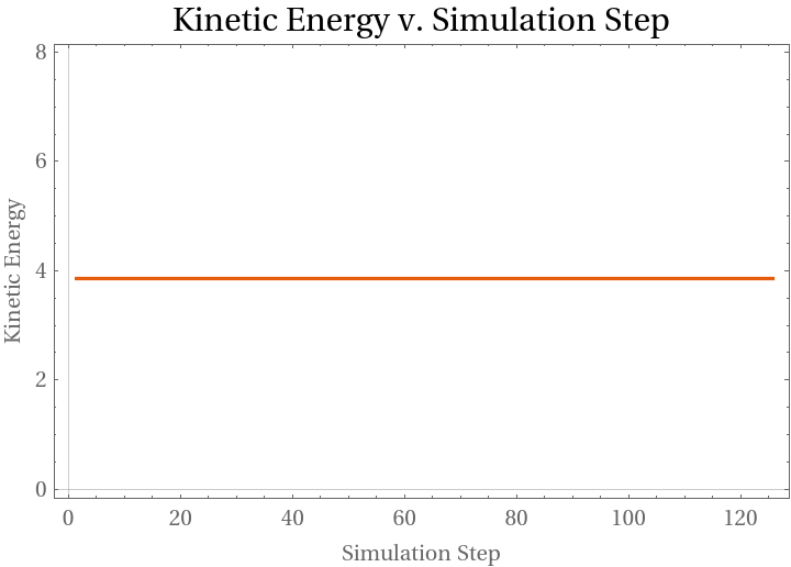Use HardSphereSimulation to simulate simplified pool:

In[13]:=

$(*Colors of pool balls*) colors = {Yellow, Blue, Red, Purple, Orange, Green, RGBColor["#800000"], Black}; (*Define graphics for stripes, solids, and cue ball*) stripes[pos_, rad_, color_, number_] := {{Black, Circle[{pos[[1]], pos[[2]]}, rad]}, {White, Disk[{pos[[1]], pos[[2]]}, 0.99 rad]}, {color, Rectangle[{pos[[1]] - 0.915 rad, pos[[2]] - 0.4 rad}, {pos[[1]] + 0.915 rad, pos[[2]] + 0.4 rad}]}, {White, Disk[{pos[[1]], pos[[2]]}, 0.3 rad]}, {color, Polygon[Table[{pos[[1]] + 0.99 rad Cos[\[Theta]], pos[[2]] + 0.99 rad Sin[\[Theta]]}, {\[Theta], -ArcTan[0.41/0.92], ArcTan[0.41/0.92], 0.005}]]}, {color, Polygon[Table[{pos[[1]] + 0.99 rad Cos[\[Theta]], pos[[2]] + 0.99 rad Sin[\[Theta]]}, {\[Theta], \[Pi] - ArcTan[0.4/0.915], \[Pi] + ArcTan[0.4/0.915], 0.01}]]}, {Text[number, pos]}}; solids[pos_, rad_, color_, number_] := {{Black, Circle[pos, rad]}, {White, Disk[pos, 0.3 rad]}, {color, Annulus[pos, {0.3 rad, 0.99 rad}]}, {Text[number, pos]}}; cue[pos_, rad_] := {{Black, Circle[pos, rad]}, {White, Disk[pos, 0.99 rad]}, {Red, Disk[pos, 0.2 rad]}};$

In[14]:=

$(*Run simulation and animate results*) Module[{traj, billiards, boxSize = 10, stepSize = 0.05, rad = 1, steps = 200}, (*Initial positions of balls in the triangle*) billiards = RandomSample[ Catenate@ Prepend[Table[ 2 row {-Cos[\[Pi]/3] + col/row, Sin[\[Pi]/3]}, {row, 1, 4}, {col, 0, row}], {{0, 0}}]]; (*Run simulation, including cue ball with small random perturbations to the break*) traj = ResourceFunction["HardSphereSimulation"][ Prepend[billiards, {0, -8} + RandomReal[{-0.1, 0.1}, 2]], Prepend[0*billiards, {0, 10} + RandomReal[{-0.1, 0.1}, 2]], boxSize, stepSize, rad, steps][[1, All, 1]]; (*Animate evolution*) Manipulate[ Graphics[ {{FaceForm[RGBColor["#0a6c03"]], EdgeForm[Black], Rectangle[{-boxSize, -boxSize}, {boxSize, boxSize}]}, cue[traj[[t, 1]], 1], Join[ Table[solids[traj[[t, n + 1]], rad, colors[[n]], n], {n, Length[colors]}], Table[ stripes[traj[[t, 8 + n + 1]], rad, colors[[n]], n + 8], {n, Length[colors] - 1}]] }, ImageSize -> 500 ], {t, 1, steps, 1}] ]$

Out[14]=

Publisher

Wolfram Summer School

Version History

2.1.0 – 30 December 2022
2.0.1 – 14 October 2022
2.0.0 – 28 September 2022
1.0.0 – 16 February 2021

Related Resources

License Information

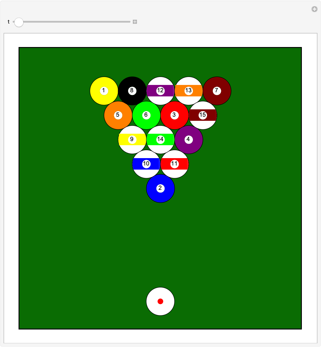This work is licensed under a Creative Commons Attribution 4.0 International License