Basic Examples (4)
Non-convex subset. The ratio measures the missing fraction of the convex hull:
A convex set has ratio zero:
Maximum fragmentation. Only boundary points remain:
The empty set returns zero:
Scope (3)
Works with rational elements:
Works with strings under canonical (lexicographic) order:
A singleton always has ratio zero:
Options (2)
The default value of "ComparisonFunction" is LessEqual:
A custom comparison function can redefine the ordering. Under the standard order 1< 2<3<4<5, the subset {1, 4} has defect ratio 0.5 because the elements 2 and 3 lie between 1 and 4:
With the custom ordering , the element 4 is the immediate successor of 1, so the interval contains only , meaning that the defect vanishes:
Default ordering. Closure of is . Two gaps. Ratio .
Custom ordering. Closure of is . Ratio 0.
Te comparison function defines the interval.
Applications (2)
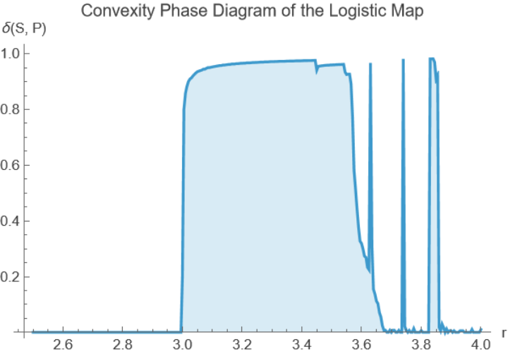
Convexity phase diagram of the logistic map
Measure the fragmentation of the logistic attractor as a function of the parameter :
For , the attractor is a fixed point and . Through the period-doubling cascade, the ratio increases as the orbit spreads into disjoint bands. The sharp dips correspond to periodic windows — intervals of stability where the orbit collapses onto a finite cycle, yielding only a few points within a wide convex hull. At , the map is conjugate to the full tent map and the orbit becomes dense in at the chosen resolution, driving .
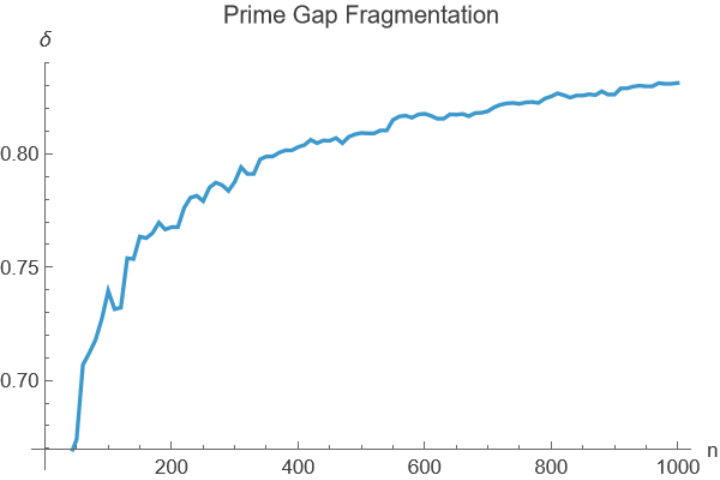
Prime gap fragmentation
The primes become maximally non-convex as , reflecting the Prime Number Theorem ( since ):
The curve increases toward 1. By the Prime Number Theorem, , so the fraction of integers that are prime within the convex hull tends to zero. Accordingly, the defect ratio approaches unity, providing a quantitative expression of the increasing sparsity of primes among the integers.
Properties and Relations (5)
The ratio is zero if and only if OrderConvexQ returns True:
Equivalent to the fraction of elements in the induced interval that are not contained in the subset:
The ratio equals one minus the density of the subset within its induced interval:
Monotonicity. Adding elements to the subset can only decrease or preserve the ratio:
A subset containing all elements of its induced interval has ratio zero:
Possible Issues (1)
Numerical precision. The result is a machine-precision real. Small rounding differences may occur compared to exact rational arithmetic.
Invalid containment. If subset is not contained in parent set, the ratio may exceed 1.
The result is a machine-precision real, not an exact rational number:
Neat Examples (2)
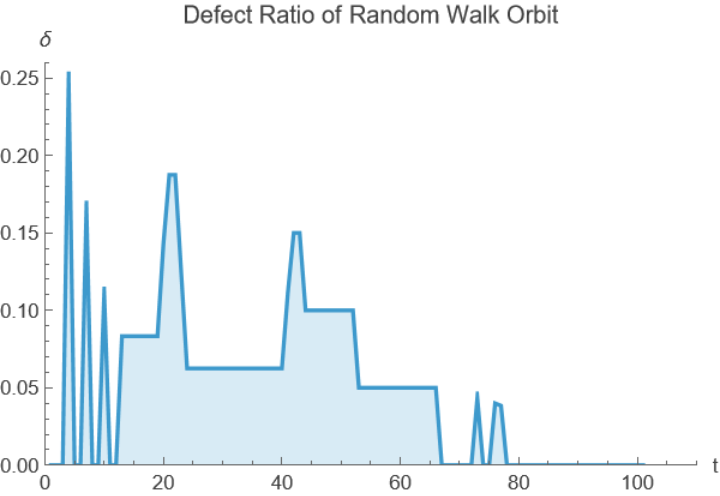
Track the defect ratio of a random walk orbit on as it explores its range over time. The ratio starts at zero (a single visited point is trivially convex), spikes as gaps appear, and eventually decays back toward zero once the walk covers every site in its range. This is a discrete analogue of the cover time on a path graph:
Compare the defect ratio across three qualitatively different dynamical regimes of the logistic map: fixed point, period-doubling, and full chaos, evaluated at representative parameter values:
The table reveals the nonmonotonic signature of the route to chaos: increases through the period-doubling cascade (), peaks inside periodic windows (e.g. , where the orbit collapses onto a low-period cycle), and returns toward zero as the attractor becomes increasingly dense, approaching full support at . The small residual value at is a finite-orbit artifact: the invariant density
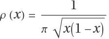
is minimal near , so this region is sampled least frequently, and the last grid points to be visited lie in that neighborhood.
![customOrd[Pattern[a,
Blank[]], Pattern[b,
Blank[]]] := Module[{order = {1, 4, 2, 5, 3}},
LessEqual[Part[Position[order, a], 1, 1],
Part[Position[order, b], 1, 1]
]
];](https://www.wolframcloud.com/obj/resourcesystem/images/a8d/a8dc85b7-7d5f-40aa-ac2a-5aa9d7b7a1e4/24b8a6d3e3f42aee.png)
![With[{grid = Range[0., 1., 0.005]},
ListLinePlot[
Table[
Module[{orbit, disc},
orbit = Part[
NestList[Function[r * # * (1 - #)], 0.2, 2000],
500 ;;
];
disc = DeleteDuplicates @ Round[orbit, 0.005];
{r, ResourceFunction["ConvexDefectRatio"][disc, grid]}
],
{r, 2.5, 4., 0.005}
],
PlotRange -> All, AxesLabel -> {"r", "\[Delta](S, P)"},
PlotLabel -> "Convexity Phase Diagram of the Logistic Map", Filling -> Bottom
]
]](https://www.wolframcloud.com/obj/resourcesystem/images/a8d/a8dc85b7-7d5f-40aa-ac2a-5aa9d7b7a1e4/725d8649b05b05a7.png)
![ListLinePlot[
Table[{n, ResourceFunction["ConvexDefectRatio"][Prime @ Range @ PrimePi @ n, Range @ n]},
{n, 10, 1000, 10}
],
AxesLabel -> {"n", "\[Delta]"},
PlotLabel -> "Prime Gap Fragmentation"
]](https://www.wolframcloud.com/obj/resourcesystem/images/a8d/a8dc85b7-7d5f-40aa-ac2a-5aa9d7b7a1e4/179a4d23cc5cbd12.png)
![With[{s = {2, 3, 5}, p = Range @ 10},
SameQ[ResourceFunction["OrderConvexQ"][s, p],
Equal[ResourceFunction["ConvexDefectRatio"][s, p], 0]
]
]](https://www.wolframcloud.com/obj/resourcesystem/images/a8d/a8dc85b7-7d5f-40aa-ac2a-5aa9d7b7a1e4/517461d8d596a073.png)
![With[{s = {1, 5, 9}, p = Range @ 10},
SameQ[ResourceFunction["ConvexDefectRatio"][s, p],
N[
Divide[
Length[
Select[p,
Function[
And[LessEqual[Min @ s, #, Max @ s], ! MemberQ[s, #]]
]
]
],
Length[Select[p, LessEqual[Min @ s, #, Max @ s] &]]
]
]
]
]](https://www.wolframcloud.com/obj/resourcesystem/images/a8d/a8dc85b7-7d5f-40aa-ac2a-5aa9d7b7a1e4/01234f172f75e35a.png)
![With[{s = {1, 4, 9}, p = Range @ 10},
SameQ[ResourceFunction["ConvexDefectRatio"][s, p],
Subtract[1,
N[
Length[s] / Length[Select[p, LessEqual[Min[s], #, Max @ s] &]]
]
]
]
]](https://www.wolframcloud.com/obj/resourcesystem/images/a8d/a8dc85b7-7d5f-40aa-ac2a-5aa9d7b7a1e4/1e5beba043815a77.png)
![With[
{
p = Range @ 20,
a = {2, 18},
b = {2, 10, 18}
},
LessEqual[ResourceFunction["ConvexDefectRatio"][b, p], ResourceFunction["ConvexDefectRatio"][a, p]]
]](https://www.wolframcloud.com/obj/resourcesystem/images/a8d/a8dc85b7-7d5f-40aa-ac2a-5aa9d7b7a1e4/76b42804c28e33f0.png)
![With[{s = {2, 8}, p = Range @ 10},
ResourceFunction["ConvexDefectRatio"][
Select[p, LessEqual[Min @ s, #, Max @ s] &], p]
]](https://www.wolframcloud.com/obj/resourcesystem/images/a8d/a8dc85b7-7d5f-40aa-ac2a-5aa9d7b7a1e4/04641a551e66e9da.png)
![SeedRandom @ 42;
Module[{walk, grid, data},
grid = Range @ 50;
walk = Clip[
Accumulate @ Prepend[RandomChoice[{-2, -1, 1, 2}, 100], 25],
{1, 50}
];
data = Table[{t, ResourceFunction["ConvexDefectRatio"][
DeleteDuplicates[walk[[1 ;; t]]], grid]},
{t, 1, 101}
];
ListLinePlot[data,
AxesLabel -> {"t", "\[Delta]"},
PlotLabel -> "Defect Ratio of Random Walk Orbit",
PlotRange -> {{0, 110}, {0, 26/100}},
Filling -> Bottom
]
]](https://www.wolframcloud.com/obj/resourcesystem/images/a8d/a8dc85b7-7d5f-40aa-ac2a-5aa9d7b7a1e4/6ac5cbdfd0bb2fbe.png)
![With[{grid = Range[0., 1., 0.001]},
TableForm[
Table[
Module[{orbit, disc},
orbit = Part[
NestList[Function[r * # * (1 - #)], 0.2, 10000],
500 ;;
];
disc = DeleteDuplicates @ Round[orbit, 0.001];
{r, Length @ disc, ResourceFunction["ConvexDefectRatio"][disc, grid]}
],
{r, {2.8, 3.2, 3.56, 3.83, 3.99, 4.}}
],
TableHeadings -> {None, {"r", "|orbit|", "\[Delta]"}}
]
]](https://www.wolframcloud.com/obj/resourcesystem/images/a8d/a8dc85b7-7d5f-40aa-ac2a-5aa9d7b7a1e4/0f32a5df92d2dc6a.png)
