Wolfram Function Repository
Instant-use add-on functions for the Wolfram Language
Function Repository Resource:
Display the regression line of a dataset
ResourceFunction["RegressionListPlot"][{y1,y2,…}] plots points {1,y1},{2,y2},… and their line of best fit. | |
ResourceFunction["RegressionListPlot"][{{x1,y1},{x2,y2},…}] plots the specified points and their regression line. | |
ResourceFunction["RegressionListPlot"][{data1,data2,…}] plots multiple datasets and their regression lines. |
Find and plot the correlation of a dataset:
| In[1]:= |
| Out[1]= | 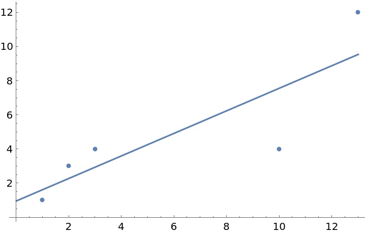 |
Generate one dataset of random numbers and one dataset of numbers correlated by a BinormalDistribution:
| In[2]:= |
Plot both of the examples datasets on the same plot:
| In[3]:= |
| Out[3]= | 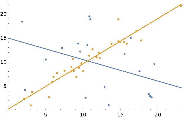 |
Specify the degree of the regression function using this option:
| In[4]:= |
| In[5]:= |
| Out[5]= | 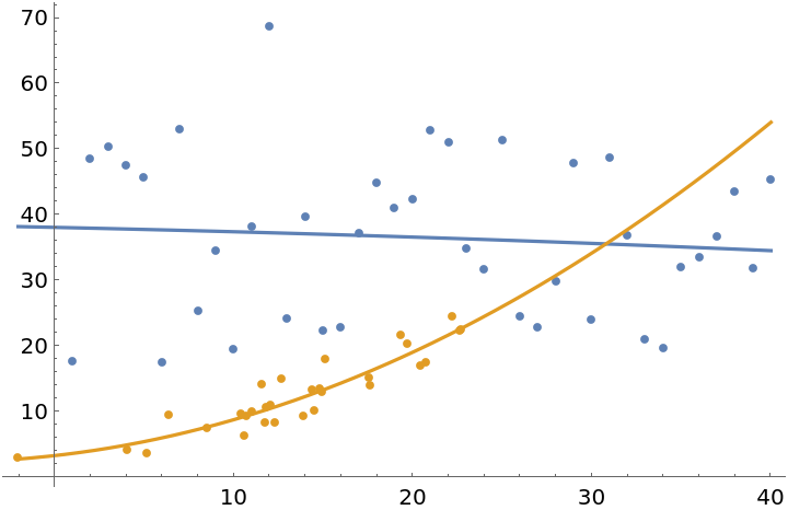 |
Degrees of multiple functions can be specified individually:
| In[6]:= |
| Out[6]= | 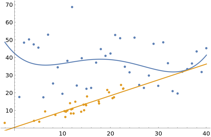 |
"DisplayEquation"→True will display the equation of the regression line:
| In[7]:= |
| Out[7]= | 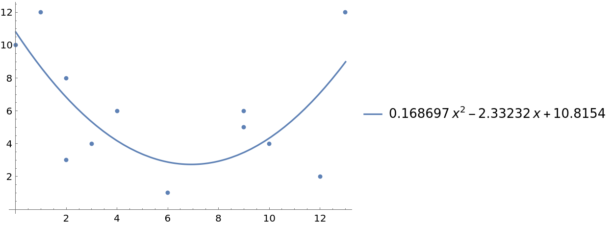 |
"DisplayRSquared" specifies whether to display the coefficient of determination. As expected, a random dataset has a much lower coefficient of determination than a related one:
| In[8]:= |
| In[9]:= |
| Out[9]= | 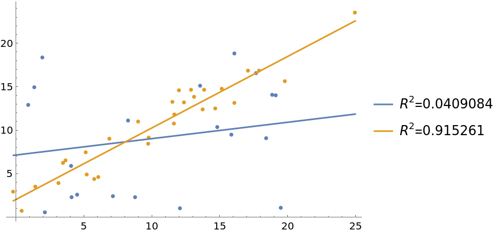 |
"DisplayRSquared" and "DisplayEquation" can both be set to True:
| In[10]:= |
| Out[10]= | 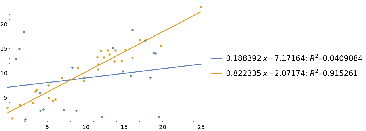 |
Correlate the current eruption duration and time to next eruption of Old Faithful geyser, October 1980:
| In[11]:= | ![ResourceFunction["RegressionListPlot"][
ExampleData[{"Statistics", "OldFaithful"}], "DisplayEquation" -> True, "DisplayRSquared" -> True, Frame -> {{True, False}, {True, False}} , FrameLabel -> {"duration of current erruption (s)", "time to next erruptions (min)"}]](https://www.wolframcloud.com/obj/resourcesystem/images/a61/a6137cfa-ddaa-430a-bbd3-c9f7605c4676/32e230f6b8f0af46.png) |
| Out[11]= | 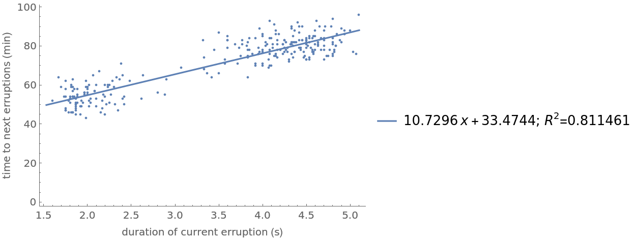 |
Visualize how sepal length, sepal width and petal length are correlated with petal width in the famous Fisher Iris dataset:
| In[12]:= | ![iris = {{#[[1]], #[[4]]} & /@ ExampleData[{"Statistics", "FisherIris"}], {#[[2]], #[[4]]} & /@ ExampleData[{"Statistics", "FisherIris"}], {#[[3]], #[[4]]} & /@ ExampleData[{"Statistics", "FisherIris"}]};](https://www.wolframcloud.com/obj/resourcesystem/images/a61/a6137cfa-ddaa-430a-bbd3-c9f7605c4676/2c49ecb45fc499c0.png) |
| In[13]:= |
| Out[13]= | 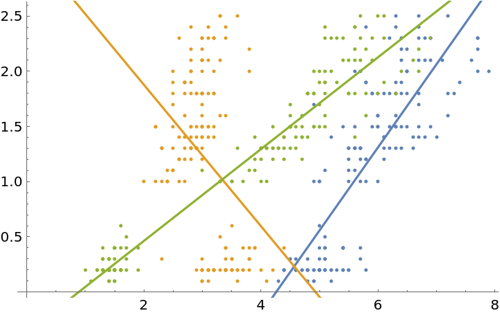 |
This work is licensed under a Creative Commons Attribution 4.0 International License