Wolfram Function Repository
Instant-use add-on functions for the Wolfram Language
Function Repository Resource:
Bin data into rectangular tiles
ResourceFunction["TileBins"][mat,s] bins a numerical full 2D array mat into square grid tiles with size s. | |
ResourceFunction["TileBins"][mat,{hx,hy}] bins a numerical full 2D array mat into rectangular grid tiles with x-y sizes {hx,hy}. | |
ResourceFunction["TileBins"][cv,s] bins coordinates-to-value rules cv. |
| "AggregationFunction" | Total | function to aggregate the data in each tile |
| "PolygonKeys" | True | determine whether the result keys are polygons |
Create a list of random 2D points:
| In[1]:= |
Bin the points:
| In[2]:= |
| Out[2]= |  |
Bin the points and get the tile centers as keys:
| In[3]:= |
| Out[3]= |
Plot points and square bins:
| In[4]:= | ![Graphics[{EdgeForm[Black], FaceForm[Opacity[0.3]], Keys@ResourceFunction["TileBins"][data, 10], Red, Point[data]}]](https://www.wolframcloud.com/obj/resourcesystem/images/7eb/7eb1f90f-4de8-42f9-82de-2edb7de5e43f/73b585a456129a27.png) |
| Out[4]= | 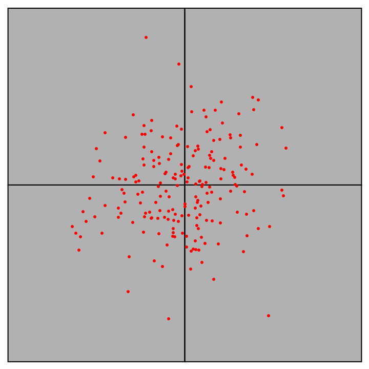 |
Plot points and rectangle bins:
| In[5]:= | ![Graphics[{EdgeForm[Black], FaceForm[Opacity[0.3]], Keys@ResourceFunction["TileBins"][data, {10, 5}], Red, Point[data]}]](https://www.wolframcloud.com/obj/resourcesystem/images/7eb/7eb1f90f-4de8-42f9-82de-2edb7de5e43f/1d5fb03a49c109c8.png) |
| Out[5]= |  |
Associate random values to 2D data:
| In[6]:= | ![SeedRandom[113];
data = RandomVariate[
MultinormalDistribution[{10, 10}, 7*IdentityMatrix[2]], 200]; dataRules = AssociationThread[data, RandomReal[{0, 1}, Length[data]]];](https://www.wolframcloud.com/obj/resourcesystem/images/7eb/7eb1f90f-4de8-42f9-82de-2edb7de5e43f/3ad111087d6426ec.png) |
Bin the data rules:
| In[7]:= |
| Out[7]= | 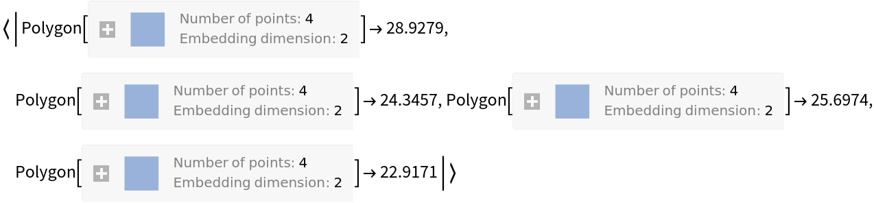 |
Bin the keys of the data rules:
| In[8]:= |
| Out[8]= | 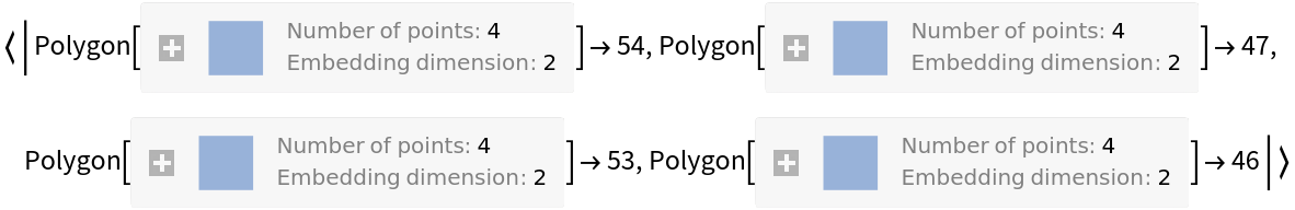 |
Check the equivalence:
| In[9]:= |
| Out[9]= |
Bin the data rules and compute average values on each tile:
| In[10]:= | ![SeedRandom[113];
data = RandomVariate[
MultinormalDistribution[{10, 10}, 7*IdentityMatrix[2]], 200]; dataRules = AssociationThread[data, RandomReal[{0, 1}, Length[data]]];
ResourceFunction["TileBins"][dataRules, 6, "AggregationFunction" -> Mean]](https://www.wolframcloud.com/obj/resourcesystem/images/7eb/7eb1f90f-4de8-42f9-82de-2edb7de5e43f/4ae6e6321e254914.png) |
| Out[10]= | 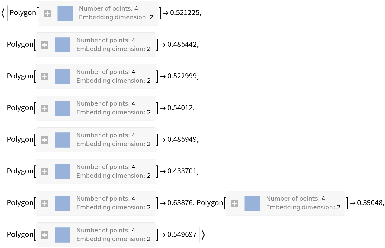 |
Compare with the default option value, Total:
| In[11]:= |
| Out[11]= | 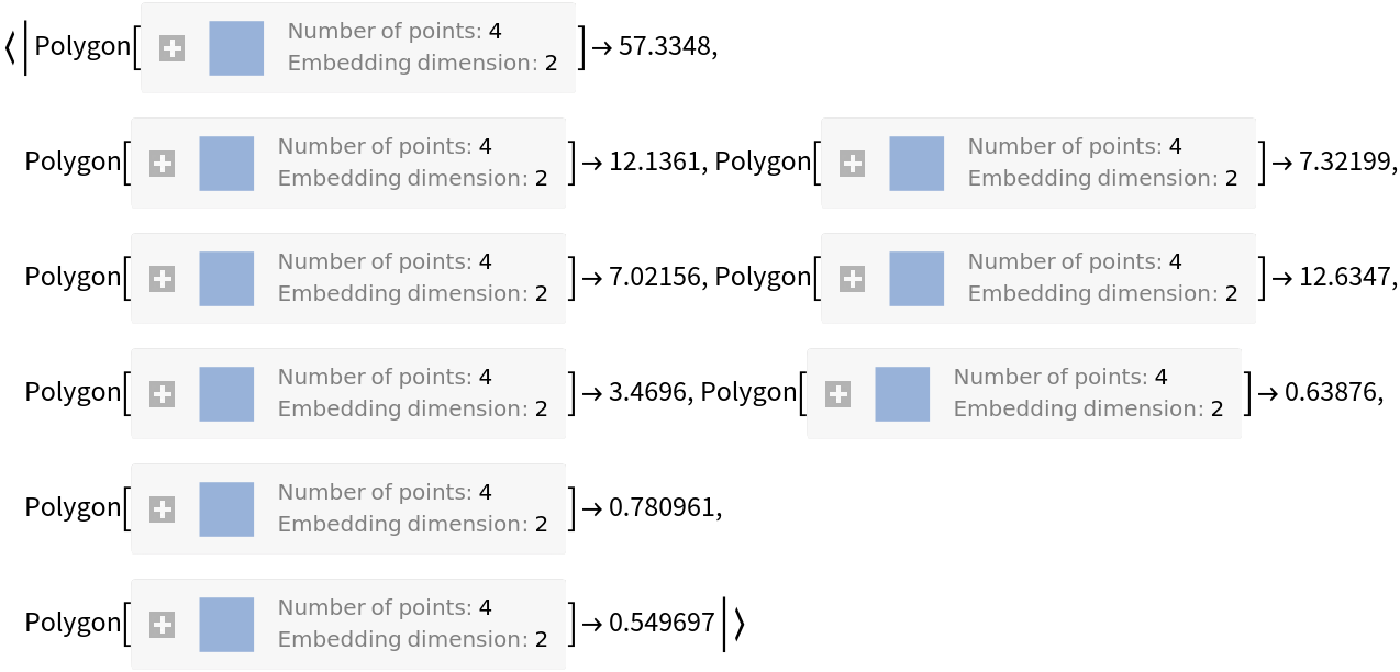 |
Instead of polygons as keys, you can get the centers of the polygons:
| In[12]:= | ![SeedRandom[113];
data = RandomVariate[
MultinormalDistribution[{10, 10}, 7*IdentityMatrix[2]], 200]; dataRules = AssociationThread[data, RandomReal[{0, 1}, Length[data]]]; ResourceFunction[
"TileBins"][dataRules, 10, "PolygonKeys" -> False]](https://www.wolframcloud.com/obj/resourcesystem/images/7eb/7eb1f90f-4de8-42f9-82de-2edb7de5e43f/51319a32b9d73376.png) |
| Out[12]= |
Generate data rules:
| In[13]:= | ![SeedRandom[113];
data2 = RandomVariate[
MultinormalDistribution[{10, 10}, 7*IdentityMatrix[2]], 300]; dataRules2 = AssociationThread[data2, RandomReal[{0, 100}, Length[data2]]];](https://www.wolframcloud.com/obj/resourcesystem/images/7eb/7eb1f90f-4de8-42f9-82de-2edb7de5e43f/401f3f37a19deb50.png) |
Here we bin the data:
| In[14]:= |
Plot points and square bins by coloring each square according to its aggregated value:
| In[15]:= | ![Graphics[{KeyValueMap[{FaceForm[
Opacity[Rescale[#2, MinMax[Values[res2]], {0, 1}], Blue]], #1} &, res2], Red, Point[Keys[dataRules2]]}, Frame -> True]](https://www.wolframcloud.com/obj/resourcesystem/images/7eb/7eb1f90f-4de8-42f9-82de-2edb7de5e43f/209d88101c119283.png) |
| Out[15]= | 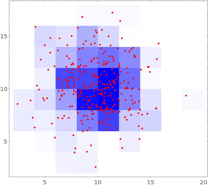 |
Repeat the visualization above with rectangular tiles instead of square ones:
| In[16]:= | ![res3 = ResourceFunction["TileBins"][
dataRules2, {4, 2}]; Graphics[{KeyValueMap[{FaceForm[
Opacity[Rescale[#2, MinMax[Values[res3]], {0, 1}], Blue]], #1} &, res3], Red, Point[Keys[dataRules2]]}, Frame -> True]](https://www.wolframcloud.com/obj/resourcesystem/images/7eb/7eb1f90f-4de8-42f9-82de-2edb7de5e43f/34870b3661e8b549.png) |
| Out[16]= | 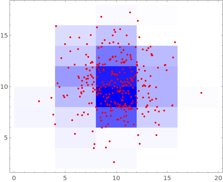 |
You can make rectangular grids:
| In[17]:= |
| Out[17]= | 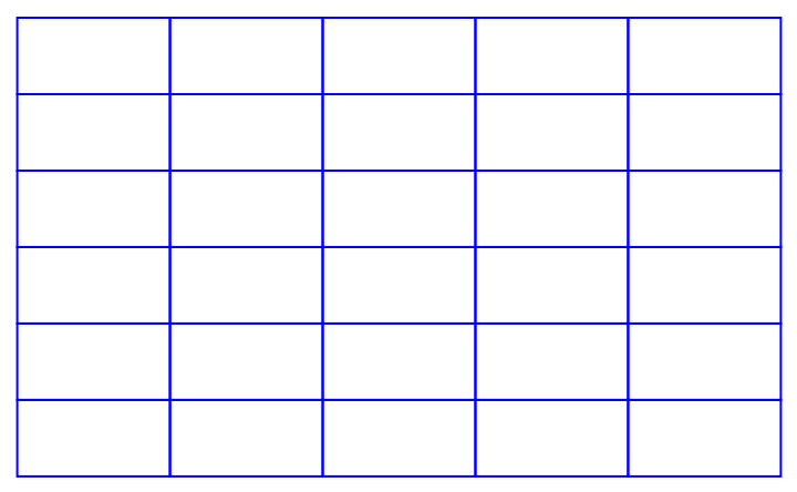 |
The coordinates of the polygons can be retrieved and transformed further:
| In[18]:= |
| Out[18]= |  |
The repository function HextileBins has similar design and implementation as TileBins. Here are comparison examples:
| In[19]:= | ![GraphicsGrid[{{Graphics[{EdgeForm[Black], FaceForm[Opacity[0.3]], Keys@ResourceFunction["HextileBins"][data, 5], Red, Point[data]},
PlotLabel -> "HextileBins"], Graphics[{EdgeForm[Black], FaceForm[Opacity[0.3]], Keys@ResourceFunction["TileBins"][data, 5], Red, Point[data]}, PlotLabel -> "TileBins"]}}]](https://www.wolframcloud.com/obj/resourcesystem/images/7eb/7eb1f90f-4de8-42f9-82de-2edb7de5e43f/21c4c62f5daaa39e.png) |
| Out[19]= | 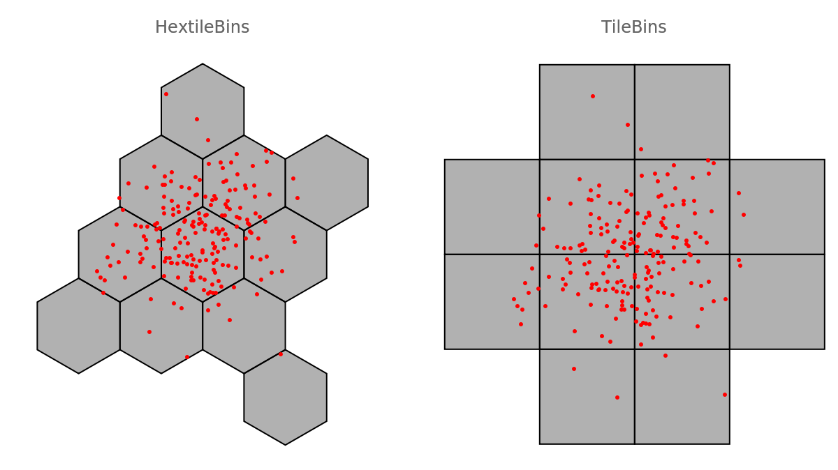 |
The function GeoHistogram produces similar plots (in Version 12.1):
| In[20]:= |
| In[21]:= |
| In[22]:= | ![geoRes = ResourceFunction["TileBins"][Reverse[#[[1]]] & /@ geoData, 0.8];
gr2 = Graphics[{KeyValueMap[{FaceForm[
Blend[{Lighter[Lighter[Yellow]], Brown}, Rescale[#2, MinMax[Values[geoRes]], {0, 1}]]], #1} &, geoRes]}, Frame -> True, Prolog -> {LightBlue, Rectangle[Scaled[{0, 0}], Scaled[{1, 1}]]},
PlotLabel -> "TileBins", ImageSize -> 250];](https://www.wolframcloud.com/obj/resourcesystem/images/7eb/7eb1f90f-4de8-42f9-82de-2edb7de5e43f/2c8ca6c58e007ed8.png) |
| In[23]:= |
| Out[23]= | 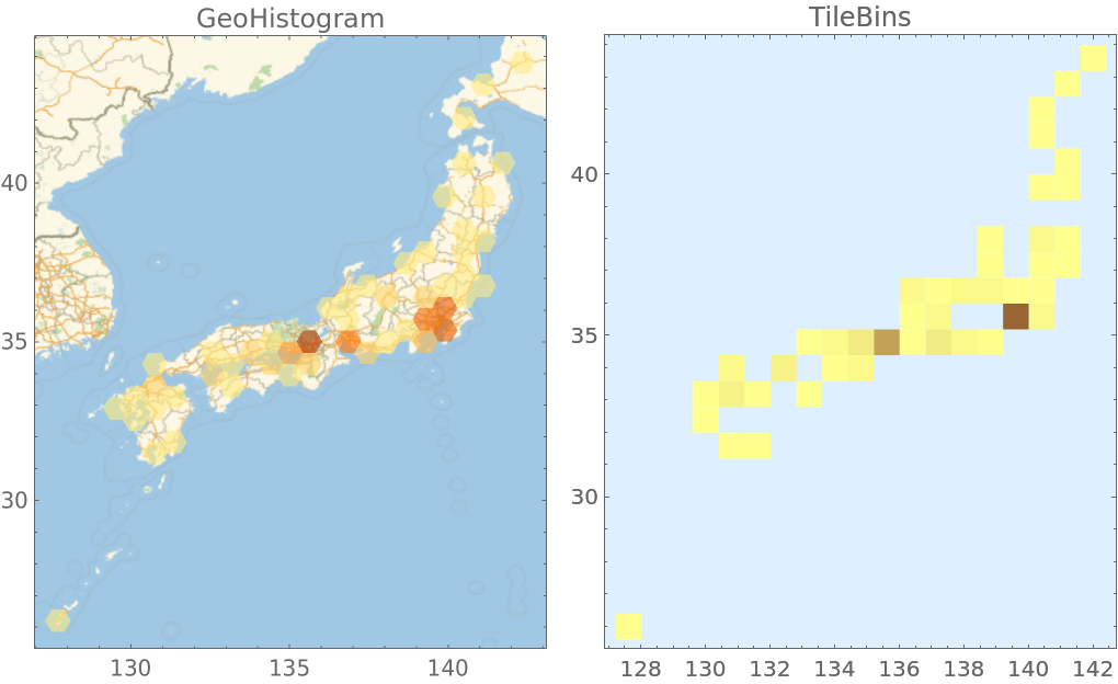 |
The function GridGraph can be also used to make rectangular grids:
| In[24]:= |
| Out[24]= | 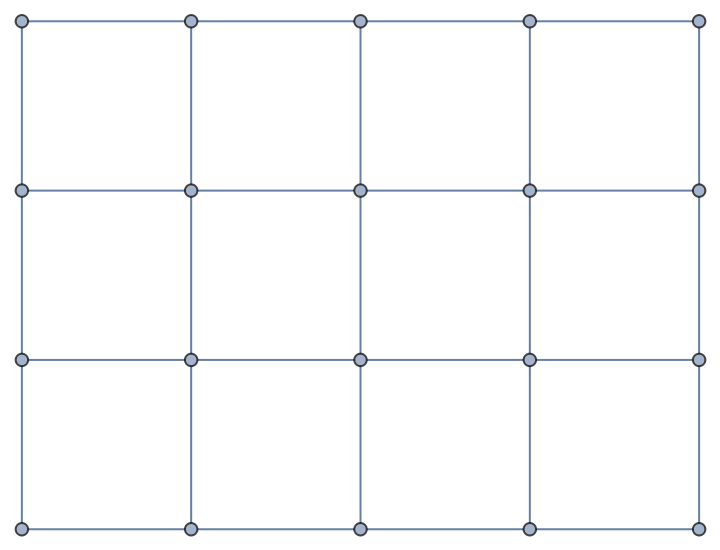 |
Here are the corresponding coordinates:
| In[25]:= |
| Out[25]= |
Here are the corresponding polygons:
| In[26]:= | ![grGridPolygons = Map[Polygon@GraphEmbedding[grGrid][[(List @@@ #)[[All, 1]]]] &, FindCycle[grGrid, {4, 4}, All]];
Graphics[{EdgeForm[Blue], FaceForm[Opacity[0.2]], grGridPolygons}]](https://www.wolframcloud.com/obj/resourcesystem/images/7eb/7eb1f90f-4de8-42f9-82de-2edb7de5e43f/561b122f9b33f16d.png) |
| Out[26]= | 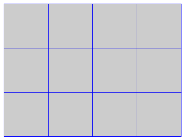 |
Make a similar grid with TileBins:
| In[27]:= |
| Out[27]= | 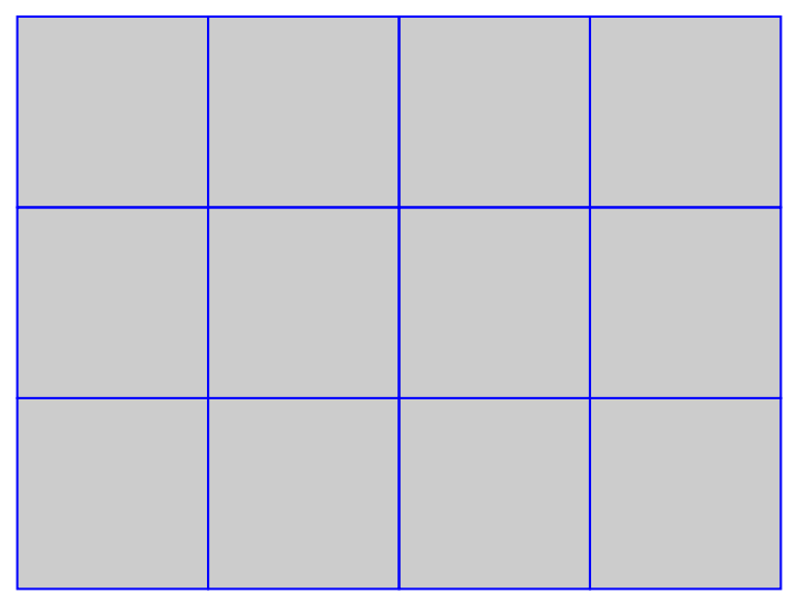 |
Here are the corresponding coordinates:
| In[28]:= |
| Out[28]= |
Bin data and summarize the values associated to bin centers:
| In[29]:= | ![SeedRandom[113];
data3 = RandomVariate[
MultinormalDistribution[{10, 10}, {1, 1.7}*IdentityMatrix[2]], 300]; dataRules3 = AssociationThread[data3, RandomReal[{0, 100}, Length[data3]]];](https://www.wolframcloud.com/obj/resourcesystem/images/7eb/7eb1f90f-4de8-42f9-82de-2edb7de5e43f/36bbe9c83522ba64.png) |
| In[30]:= |
| Out[30]= | 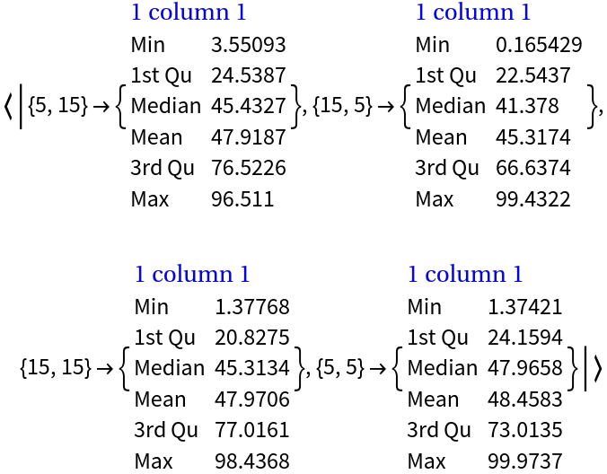 |
This work is licensed under a Creative Commons Attribution 4.0 International License