Details
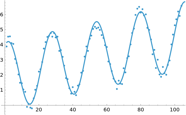
The model was first introduced by Robert E. Serfling in 1963[1] to track baseline influenza-related infection by analysing the seasonal patterns of disease spread. The model takes the following general form:
where the first component is a polynomial function of degree
d and the second component consists of
r pairs of sine-cosine functions to resemble seasonal patterns. Originally, Serfling introduced it with
d=r=1 however additional sine-cosine pairs can be added to reflect specific periodic patterns.
The coefficients ai, si and ci are the regression coefficients whereas the ωi are the periods of seasonal patterns. For example, if infection occurs twice each year, then a single pair of sine-cosine functions with ω1=26 (in weeks, assuming data is weekly) can suffice. However, if infection tends to peak more sharply in one season as compared to the other, adding an additional pair of sine and cosine functions with ω2=52 (say) can help reflect this annual pattern more accurately.
The data should be a list of target values yi or a list of (ti,yi) tuples. A list of omegas should correspond to the pairs of sine-cosine functions needed in the model described above.
Ordinarily, d=1 (linear polynomial) suffices, however additional polynomial terms can be added such as a2t2 to model population growth, if needed.
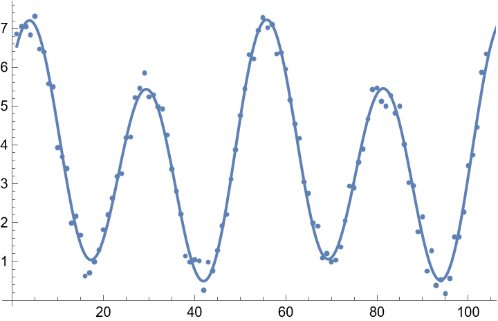
![data = Table[{t, 2 + 0.025 t + 2 Cos[(2 Pi t)/26] + Sin[(2 Pi t)/26] + RandomReal[{-0.5, 0.5}]}, {t, 104}];
ListPlot[data]](https://www.wolframcloud.com/obj/resourcesystem/images/357/3570b177-b521-4950-a76e-c5ce6839f53e/3a7877b8503f9bcb.png)
![Show[
ListPlot[data],
Plot[fit[t], {t, 1, 120}]
]](https://www.wolframcloud.com/obj/resourcesystem/images/357/3570b177-b521-4950-a76e-c5ce6839f53e/774a4d665cb0d9ee.png)
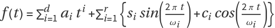
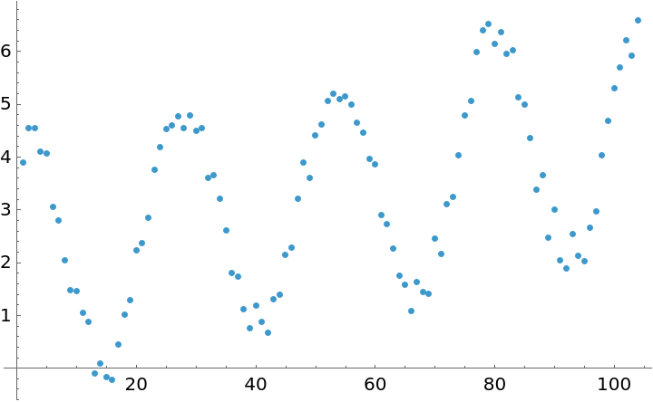
![data = Table[{t, 3.5 + 0.001 t + 1.8 Cos[(2 Pi t)/26] + 2.1 Sin[(2 Pi t)/26] + 0.7 Cos[(2 Pi t)/52] + 0.6 Sin[(2 Pi t)/52] + RandomReal[{-0.5, 0.5}]}, {t, 104}];](https://www.wolframcloud.com/obj/resourcesystem/images/357/3570b177-b521-4950-a76e-c5ce6839f53e/1079255f2c59895f.png)
![Show[
ListPlot[data],
Plot[fit[t], {t, 1, 120}]
]](https://www.wolframcloud.com/obj/resourcesystem/images/357/3570b177-b521-4950-a76e-c5ce6839f53e/1d4d853cab176651.png)