Wolfram Function Repository
Instant-use add-on functions for the Wolfram Language
Function Repository Resource:
Compute the polar radius of a regular polygon
ResourceFunction["RegularPolygonAngleRadius"][t,n] computes the polar radius at angle t with respect to the x axis of a regular polygon with n vertices equally spaced around the unit circle. | |
ResourceFunction["RegularPolygonAngleRadius"][t,r,n] computes the radius of a regular polygon whose vertices lie on a circle of radius r. | |
ResourceFunction["RegularPolygonAngleRadius"][t,t0,r,n] starts at angle t0 with respect to the x axis. |
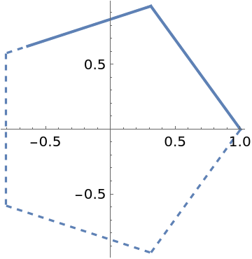
Draw the perimeter of a regular polygon using polar coordinates:
| In[1]:= |
![With[{n = 5}, Show[MapThread[
PolarPlot[
ResourceFunction["RegularPolygonAngleRadius"][t, n], {t, 0, #1}, PlotStyle -> #2, ImageSize -> Small] &, {{3 \[Pi]/4, 2 \[Pi]}, {Thick, Dashed}}]]]](https://www.wolframcloud.com/obj/resourcesystem/images/0dc/0dc6149a-1b2f-4db7-9e67-7b7587415a9d/3d09802b9a8eb272.png)
|
| Out[1]= |
|
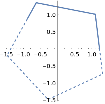
Use a different radius and starting angle:
| In[2]:= |
![With[{n = 5, t0 = 0.75, r = 1.5}, Show[MapThread[
PolarPlot[
ResourceFunction["RegularPolygonAngleRadius"][t, t0, r, n], {t, 0, #1}, PlotStyle -> #2, ImageSize -> Small] &, {{3 \[Pi]/4, 2 \[Pi]}, {Thick, Dashed}}]]]](https://www.wolframcloud.com/obj/resourcesystem/images/0dc/0dc6149a-1b2f-4db7-9e67-7b7587415a9d/70865d6d769b0019.png)
|
| Out[2]= |
|
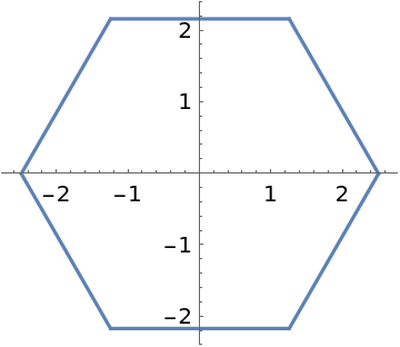
Draw the perimeter of any regular polygon using parametric coordinates:
| In[3]:= |
![With[{n = 6, t0 = 0, r = 2.5}, ParametricPlot[
AngleVector[{ResourceFunction["RegularPolygonAngleRadius"][t, t0, r,
n], t}], {t, 0, 2 \[Pi]}, ImageSize -> Small]]](https://www.wolframcloud.com/obj/resourcesystem/images/0dc/0dc6149a-1b2f-4db7-9e67-7b7587415a9d/512e84d4aaf0963c.png)
|
| Out[3]= |
|
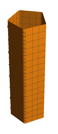
Construct a cylinder with a polygonal cross-section:
| In[4]:= |
![ParametricPlot3D[
Insert[AngleVector[{ResourceFunction["RegularPolygonAngleRadius"][t, 0, 1, 5], t}], v, -1], {t, 0, 2 \[Pi]}, {v, -3, 3}, Axes -> False, Boxed -> False, Exclusions -> None, WorkingPrecision -> 20, PerformanceGoal -> "Quality", ImageSize -> Small]](https://www.wolframcloud.com/obj/resourcesystem/images/0dc/0dc6149a-1b2f-4db7-9e67-7b7587415a9d/050f55ac8ad1da91.png)
|
| Out[4]= |
|
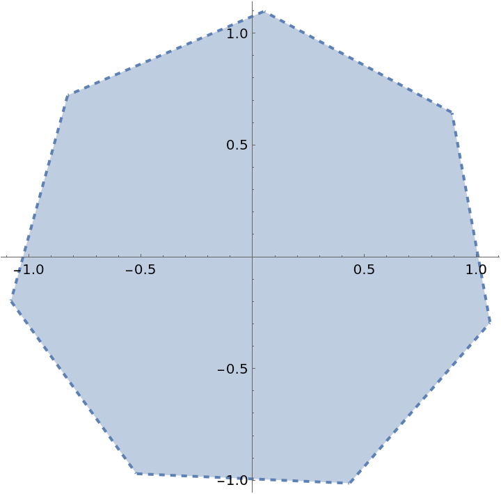
RegularPolygonAngleRadius gives the boundary of RegularPolygon:
| In[5]:= |
![With[{t0 = \[Pi]/5, r = 1.1, n = 7}, PolarPlot[
ResourceFunction["RegularPolygonAngleRadius"][t, t0, r, n], {t, 0, 2 \[Pi]}, PlotStyle -> Directive[Dashed, Thick], Prolog -> {Directive[Opacity[0.4], ColorData[97, 1]], RegularPolygon[{r, t0}, n]}]]](https://www.wolframcloud.com/obj/resourcesystem/images/0dc/0dc6149a-1b2f-4db7-9e67-7b7587415a9d/2ceda946677615e6.png)
|
| Out[5]= |
|
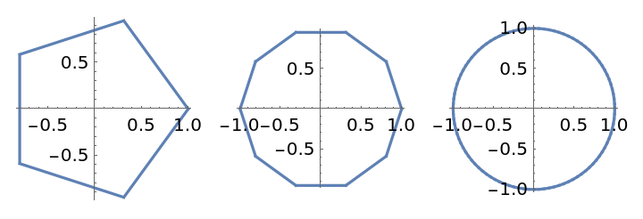
With n very large (>100), one gets an approximation to a circle:
| In[6]:= |
![GraphicsRow[
PolarPlot[
ResourceFunction["RegularPolygonAngleRadius"][t, 0, 1, #], {t, 0, 2 \[Pi]}, ImageSize -> Small] & /@ {5, 10, 100}, ImageSize -> Medium]](https://www.wolframcloud.com/obj/resourcesystem/images/0dc/0dc6149a-1b2f-4db7-9e67-7b7587415a9d/3cb79fab43f5b50d.png)
|
| Out[6]= |
|
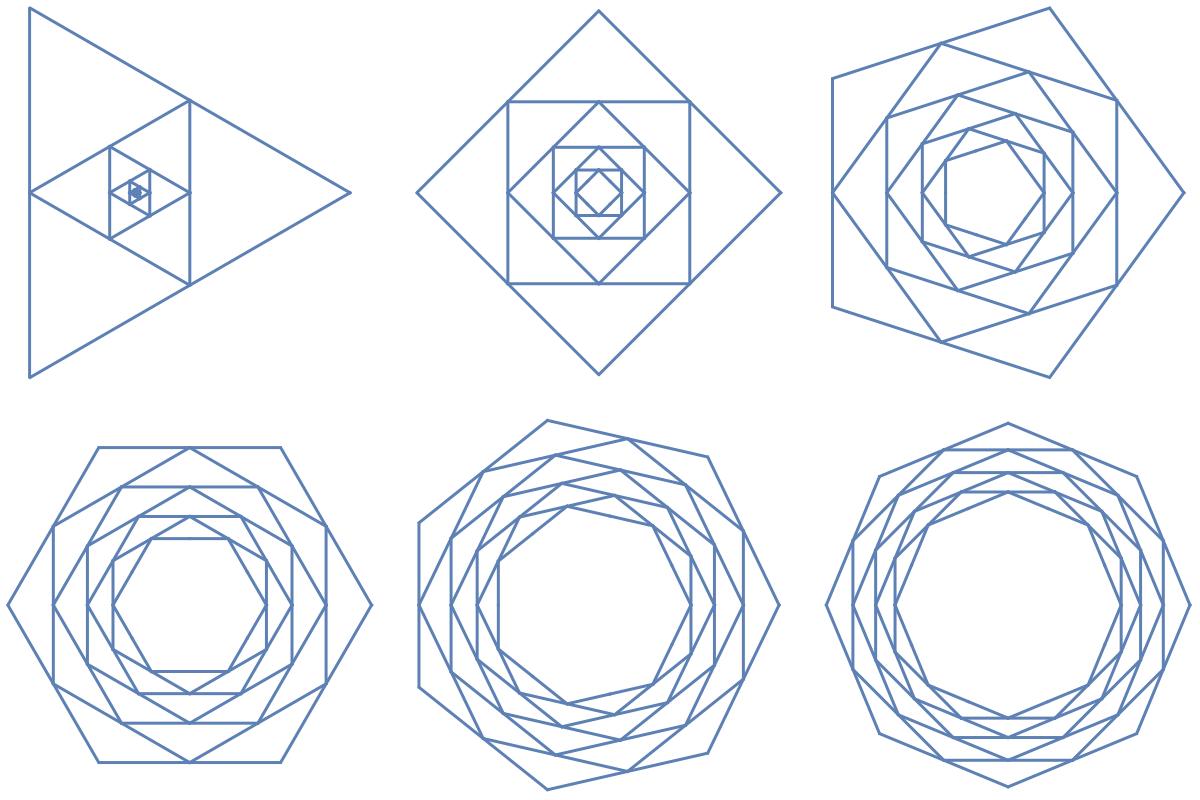
This work is licensed under a Creative Commons Attribution 4.0 International License
![With[{p = 6}, Partition[
Table[PolarPlot[
Table[ResourceFunction["RegularPolygonAngleRadius"][
t, \[Pi]/n Mod[k, 2], Cos[\[Pi]/n]^k, n], {k, 0, p}] // Evaluate, {t, 0, 2 \[Pi]}, Axes -> None, PlotRange -> All, PlotStyle -> Directive[AbsoluteThickness[1.5], ColorData[97, 1]]], {n, 3, 8}], 3]] // GraphicsGrid](https://www.wolframcloud.com/obj/resourcesystem/images/0dc/0dc6149a-1b2f-4db7-9e67-7b7587415a9d/5070a84ad4eb79e5.png)
![With[{n = 9}, PolarPlot[Flatten[Table[{\!\(
\*UnderoverscriptBox[\(\[Product]\), \(j = 3\), \(k - 1\)]\(Sec[
\*FractionBox[\(\[Pi]\), \(j\)]]\)\), ResourceFunction["RegularPolygonAngleRadius"][t, 0, \!\(
\*UnderoverscriptBox[\(\[Product]\), \(j = 3\), \(k\)]\(Sec[
\*FractionBox[\(\[Pi]\), \(j\)]]\)\), k]}, {k, 3, n}]] // Evaluate, {t, 0, 2 \[Pi]}, Axes -> None, PlotPoints -> 75, PlotRange -> All, PlotStyle -> Directive[AbsoluteThickness[1.5], ColorData[97, 1]]]]](https://www.wolframcloud.com/obj/resourcesystem/images/0dc/0dc6149a-1b2f-4db7-9e67-7b7587415a9d/029dc9ebe63a424a.png)