Wolfram Function Repository
Instant-use add-on functions for the Wolfram Language
Function Repository Resource:
Represent a discrete quantum state
ResourceFunction["QuantumDiscreteState"][<|b1→amp1,b2→amp2,…|>,purity,QuantumBasis[…]] represents a discrete quantum state with basis elements bi and associated amplitudes ampi, with purity purity, defined with respect to a specified QuantumBasis. | |
ResourceFunction["QuantumDiscreteState"][{amp1,amp2,…},QuantumBasis[…]] represents a (pure) discrete quantum state with state vector {amp1,amp2,…}, defined with respect to a specified QuantumBasis. | |
ResourceFunction["QuantumDiscreteState"][mat,QuantumBasis[…]] represents a (generically mixed) discrete quantum state with density matrix mat, defined with respect to a specified QuantumBasis. | |
ResourceFunction["QuantumDiscreteState"]["name",pic] represents a named discrete quantum state "name", with respect to the quantum mechanical picture pic. | |
ResourceFunction["QuantumDiscreteState"][{"name",n},pic] represents an n-qudit version of a named discrete quantum state "name", with respect to the quantum mechanical picture pic. | |
ResourceFunction["QuantumDiscreteState"][ResourceFunction["QuantumDiscreteState"][…],QuantumBasis[…]] transforms a specified ResourceFunction["QuantumDiscreteState"] into a new QuantumBasis. | |
ResourceFunction["QuantumDiscreteState"][ResourceFunction["QuantumDiscreteState"][…],pic] transforms a specified ResourceFunction["QuantumDiscreteState"] into the new quantum mechanical picture pic. |
| "Amplitudes" | association <|b1→amp1,b2→amp2,…|> of basis names and amplitudes |
| "Basis" | which QuantumBasis the state is defined with respect to |
| "Picture" | which quantum mechanical picture the state is defined with respect to |
| "BasisElements" | list of basis elements bi |
| "StateVector" | state vector {amp1,amp2,…} (for pure states only) |
| "DensityMatrix" | density matrix mat (for both pure and mixed states) |
| "VonNeumannEntropy" | Von Neumann entropy (entanglement entropy) of the state |
| "Purity" | purity of the quantum state, specified as a real number |
| "PureStateQ" | whether the state is pure (purity equals 1) |
| "MixedStateQ" | whether the state is mixed (purity is not equal to 1) |
| "Qudits" | number of qudits (subsystems) within the state |
| "Dimensions" | dimensionality of each qudit (subsystem) |
| "BlochSphericalCoordinates" | spherical coordinates of the state on the Bloch sphere (qubits only) |
| "BlochCartesianCoordinates" | Cartesian coordinates of the state on the Bloch sphere (qubits only) |
| "BlochPlot" | plot the state on the Bloch sphere (qubits only) |
| "Properties" | list of all property names |
| "Plus" | positive x-basis state |+〉 on the Bloch sphere |
| "Minus" | negative x-basis state |-〉 on the Bloch sphere |
| "Left" | positive y-basis state |L〉 on the Bloch sphere |
| "Right" | negative y-basis state |R〉 on the Bloch sphere |
| "PhiPlus" | maximally-entangled Bell state |Φ+〉 |
| "PhiMinus" | maximally-entangled Bell state |Φ-〉 |
| "PsiPlus" | maximally-entangled Bell state |Ψ+〉 |
| "PsiMinus" | maximally-entangled Bell state |Ψ-〉 |
| {"BasisState",list} | composite computational basis state consisting of a tensor product of single-qudit computational basis states from list |
| {"Register",n} | quantum register consisting of n qudits in the 0th computational basis state |
| {"Register",n,i} | quantum register consisting of n qudits in the ith computational basis state |
| "UniformSuperposition" | uniform superposition of a single qudit |
| {"UniformSuperposition",n} | uniform superposition of n qudits |
| "RandomPure" | random pure state for a single qudit |
| {"RandomPure",n} | random pure state for n qudits |
| "GHZ" | maximally-entangled Greenberger–Horne–Zeilinger state for 3 qudits |
| {"GHZ",n} | maximally-entangled Greenberger–Horne–Zeilinger state for n qudits |
| "W" | entangled W state for 3 qudits |
| {"W",n} | entangled W state for n qudits |
| "Werner" | bipartite Werner state for 2 qubits with relative weight equal to 0 |
| {"Werner",ρ} | bipartite Werner state for 2 qubits with relative weight equal to ρ |
| {"Graph",g} | multi-qubit graph state specified by g |
Create a pure discrete quantum state from a state vector in the computational basis (default):
| In[1]:= |
| Out[1]= |
Return its amplitude association (automatically normalized):
| In[2]:= |
| Out[2]= |
Return its density matrix:
| In[3]:= |
| Out[3]= |
Plot the state on the Bloch sphere:
| In[4]:= |
| Out[4]= | 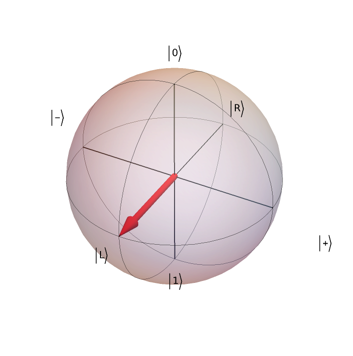 |
Create a mixed discrete quantum state from a density matrix in the computational basis:
| In[5]:= |
| Out[5]= |
Show that the state is not pure:
| In[6]:= |
| Out[6]= |
| In[7]:= |
| Out[7]= |
Return its von Neumann entropy:
| In[8]:= |
| Out[8]= |
Plot the state on the Bloch sphere:
| In[9]:= |
| Out[9]= |  |
Create a pure discrete quantum state by explicitly specifying an association of amplitudes in a given basis:
| In[10]:= | ![state = ResourceFunction[
"QuantumDiscreteState"][<|"up" -> 1 + 3 I, "down" -> 2 - 4 I|>, "Pure", ResourceFunction["QuantumBasis"][<|"up" -> {1, 0}, "down" -> {0, 1}|>]]](https://www.wolframcloud.com/obj/resourcesystem/images/630/63062f3f-ef64-497d-aa44-fad03a13b339/15cab054301beb0d.png) |
| Out[10]= |
Return its state vector (automatically normalized):
| In[11]:= |
| Out[11]= |
Return its basis element association:
| In[12]:= |
| Out[12]= |
Return the spherical coordinates of the state on the Bloch sphere:
| In[13]:= |
| Out[13]= |
Return the Cartesian coordinates of the state on the Bloch sphere:
| In[14]:= |
| Out[14]= |
Create a maximally-entangled GHZ state for 3 qubits (default):
| In[15]:= |
| Out[15]= |
| In[16]:= |
| Out[16]= |  |
Create a maximally-entangled GHZ state for 4 qubits instead:
| In[17]:= |
| Out[17]= |
| In[18]:= |
| Out[18]= | 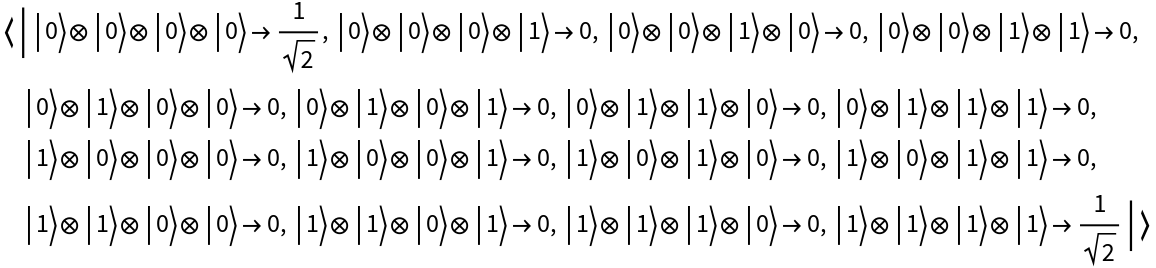 |
By default, all discrete quantum states are assumed to consist of tensor products of 2-dimensional subsystems (i.e. qubits):
| In[19]:= |
| Out[19]= |
| In[20]:= |
| Out[20]= |
Create a discrete quantum state with the same state vector consisting of a single 4-dimensional subsystem (i.e. a qudit) instead:
| In[21]:= |
| Out[21]= |
| In[22]:= |
| Out[22]= |
Create a pure discrete quantum state in the computational basis (default):
| In[23]:= |
| Out[23]= |
| In[24]:= |
| Out[24]= |
| In[25]:= |
| Out[25]= |
Transform the state to the Fourier basis:
| In[26]:= |
| Out[26]= |
| In[27]:= |
| Out[27]= |
| In[28]:= |
| Out[28]= |
Transform the state back to the computational basis:
| In[29]:= |
| Out[29]= |
| In[30]:= |
| Out[30]= |
| In[31]:= |
| Out[31]= |
The initial and final states are the same:
| In[32]:= |
| Out[32]= |
Represent the maximally-entangled "PhiPlus" Bell basis state in the Heisenberg picture:
| In[33]:= |
| Out[33]= |
| In[34]:= |
| Out[34]= |
Transform the state to the interaction picture:
| In[35]:= |
| Out[35]= |
| In[36]:= |
| Out[36]= |
Mixed states do not have state vector representations—only density matrix representations:
| In[37]:= |
| Out[37]= |
| In[38]:= |
| Out[38]= |
| In[39]:= |
| Out[39]= |
Return its amplitude association:
| In[40]:= |
| Out[40]= |
Return its purity:
| In[41]:= |
| Out[41]= |
On the other hand, pure states have both state vector and density matrix representations:
| In[42]:= |
| Out[42]= |
| In[43]:= |
| Out[43]= |
| In[44]:= |
| Out[44]= |
Return its purity:
| In[45]:= |
| Out[45]= |
Create a 3-qubit random pure quantum state in the computational basis:
| In[46]:= |
| Out[46]= |
| In[47]:= |
| Out[47]= |  |
| In[48]:= |
| Out[48]= |
Represent the same state in the Pauli-X basis instead:
| In[49]:= |
| Out[49]= |
| In[50]:= |
| Out[50]= |  |
| In[51]:= |
| Out[51]= |
Represent the orthonormal x- and y-basis states on the Bloch sphere:
| In[52]:= |
| Out[52]= | 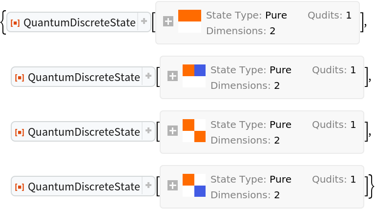 |
| In[53]:= |
| Out[53]= |
Represent the maximally-entangled Bell basis states for 2 qubits:
| In[54]:= |
| Out[54]= | 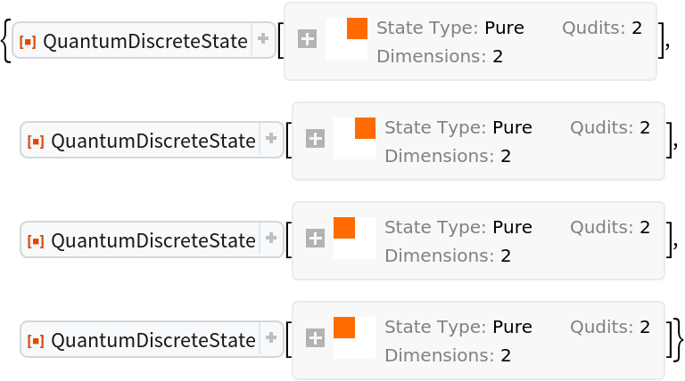 |
| In[55]:= |
| Out[55]= |  |
Represent the {0,1} computational basis state for a pair of 2 qubits:
| In[56]:= |
| Out[56]= |
| In[57]:= |
| Out[57]= |
Represent the {2,2,1,1} computational basis state for a 4-tuple of 3-dimensional qudits:
| In[58]:= |
| Out[58]= |
| In[59]:= |
| Out[59]= | 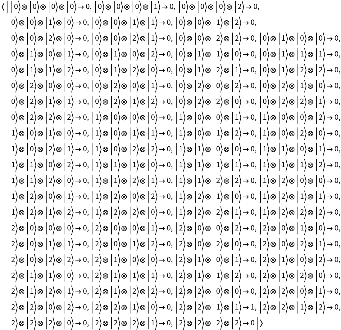 |
Represent a 3-qubit quantum register in the 0th computational basis state:
| In[60]:= |
| Out[60]= |
| In[61]:= |
| Out[61]= |
Represent a 3-qubit quantum register in the 4th computational basis state:
| In[62]:= |
| Out[62]= |
| In[63]:= |
| Out[63]= |
Represent a quantum register consisting of 2 3-dimensional qudits in the 4th computational basis state:
| In[64]:= |
| Out[64]= |
| In[65]:= |
| Out[65]= |
Represent a uniform superposition state for a single qubit:
| In[66]:= |
| Out[66]= |
| In[67]:= |
| Out[67]= |
Represent a uniform superposition state for 3 qubits:
| In[68]:= |
| Out[68]= |
| In[69]:= |
| Out[69]= | 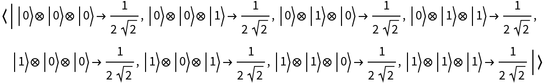 |
Represent a uniform superposition state for 2 3-dimensional qudits:
| In[70]:= |
| Out[70]= |
| In[71]:= |
| Out[71]= |  |
Represent a random pure state for a single qubit:
| In[72]:= |
| Out[72]= |
| In[73]:= |
| Out[73]= |
Represent a random pure state for 3 qubits:
| In[74]:= |
| Out[74]= |
| In[75]:= |
| Out[75]= |  |
Represent a random pure state for 2 3-dimensional qudits:
| In[76]:= |
| Out[76]= |
| In[77]:= |
| Out[77]= | 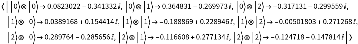 |
Represent the maximally-entangled GHZ state for 3 qubits:
| In[78]:= |
| Out[78]= |
| In[79]:= |
| Out[79]= |  |
Represent the maximally-entangled GHZ state for 4 qubits:
| In[80]:= |
| Out[80]= |
| In[81]:= |
| Out[81]= |  |
Represent the maximally-entangled GHZ state for 3 3-dimensional qudits:
| In[82]:= |
| Out[82]= |
| In[83]:= |
| Out[83]= |  |
Represent the entangled W state for 3 qubits:
| In[84]:= |
| Out[84]= |
| In[85]:= |
| Out[85]= |  |
Represent the entangled W state for 4 qubits:
| In[86]:= |
| Out[86]= |
| In[87]:= |
| Out[87]= | 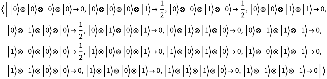 |
Represent the entangled W state for 3 3-dimensional qudits:
| In[88]:= |
| Out[88]= |
| In[89]:= |
| Out[89]= | 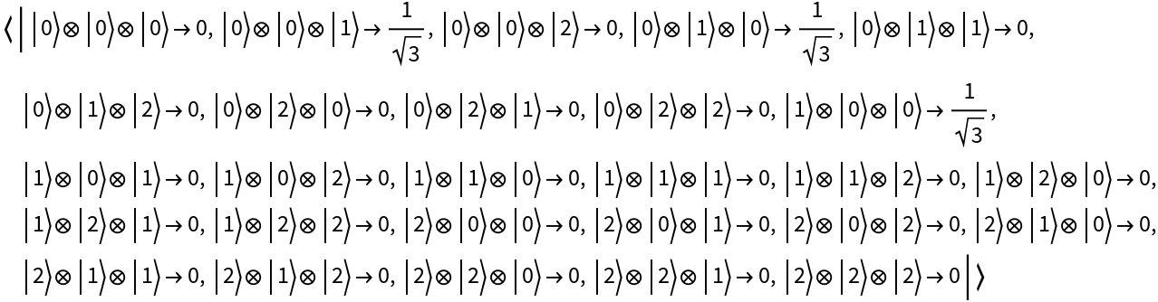 |
Represent the bipartite Werner state for 2 qubits, with relative weight equal to 0 (default):
| In[90]:= |
| Out[90]= |
| In[91]:= |
| Out[91]= |
| In[92]:= |
| Out[92]= |  |
Return its purity:
| In[93]:= |
| Out[93]= |
Represent the bipartite Werner state for 2 qubits, with relative weight equal to 0.5:
| In[94]:= |
| Out[94]= |
| In[95]:= |
| Out[95]= |
| In[96]:= |
| Out[96]= | 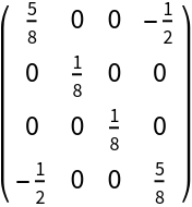 |
Return its von Neumann entropy:
| In[97]:= |
| Out[97]= |
Represent the 3-qubit graph state described by a 3-vertex path graph:
| In[98]:= |
| Out[98]= |
| In[99]:= |
| Out[99]= |
| In[100]:= |
| Out[100]= | 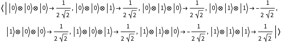 |
Represent the 3-qubit graph state described by a 3-vertex triangle graph:
| In[101]:= |
| Out[101]= | 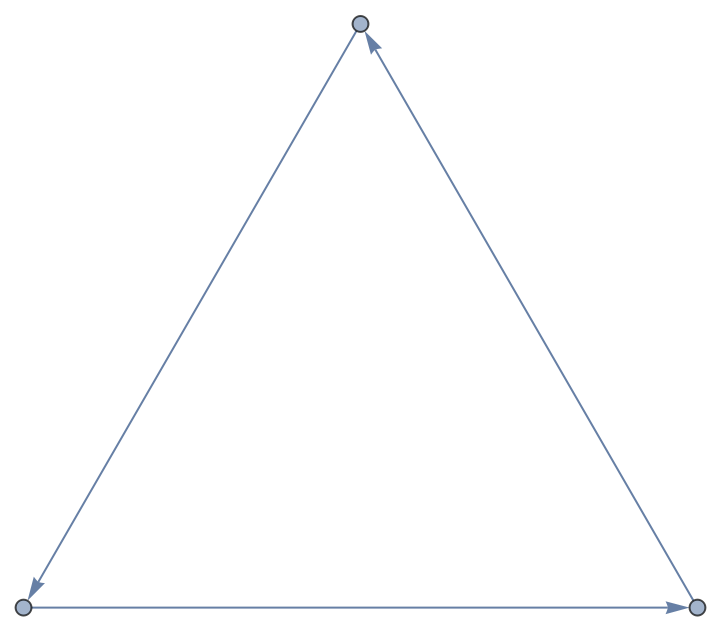 |
| In[102]:= |
| Out[102]= |
| In[103]:= |
| Out[103]= | 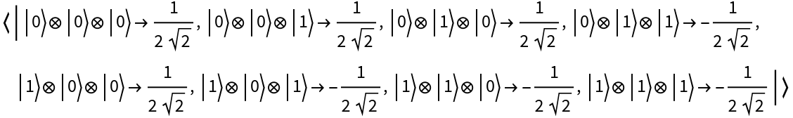 |
QuantumDiscreteState objects can be constructed purely symbolically (without explicit vector or matrix elements):
| In[104]:= |
| Out[104]= |
View the amplitude association:
| In[105]:= |
| Out[105]= |
Standard operations can still be performed on purely symbolic states:
| In[106]:= |
| Out[106]= |
| In[107]:= |
| Out[107]= |
View a list of properties that can be extracted from a QuantumDiscreteState object:
| In[108]:= |
| Out[108]= |
| In[109]:= |
| Out[109]= |
Return the association of amplitudes:
| In[110]:= |
| Out[110]= |
Return which QuantumBasis the state is defined with respect to:
| In[111]:= |
| Out[111]= |
Return which quantum mechanical picture the state is defined with respect to:
| In[112]:= |
| Out[112]= |
Return the association of names and basis elements:
| In[113]:= |
| Out[113]= |
Return the state vector:
| In[114]:= |
| Out[114]= |
Return the density matrix:
| In[115]:= |
| Out[115]= |
Return the von Neumann entropy (0 for pure states):
| In[116]:= |
| Out[116]= |
Return the purity (1 for pure states):
| In[117]:= |
| Out[117]= |
Determine whether the state is pure:
| In[118]:= |
| Out[118]= |
Determine whether the state is mixed:
| In[119]:= |
| Out[119]= |
Return the number of qudits (subsystems):
| In[120]:= |
| Out[120]= |
Return the number of dimensions:
| In[121]:= |
| Out[121]= |
Return the spherical coordinates of the state on the Bloch sphere:
| In[122]:= |
| Out[122]= |
Return the Cartesian coordinates of the state on the Bloch sphere:
| In[123]:= |
| Out[123]= |
Plot the state on the Bloch sphere:
| In[124]:= |
| Out[124]= | 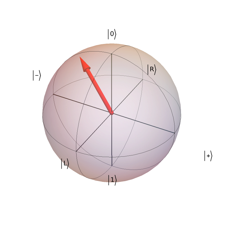 |
This work is licensed under a Creative Commons Attribution 4.0 International License