Wolfram Function Repository
Instant-use add-on functions for the Wolfram Language
Function Repository Resource:
Get the roots of a derivative for applying the Lucas–Gauss theorem on a set of points
ResourceFunction["PointsetDerivativeRoots"][pts] applies the Lucas-Gauss derivative on a set of pts and finds the roots. |
Find the roots of a set of points:
| In[1]:= | ![pts = {{Sqrt[6], 1}, {-Sqrt[6], 1}, {0, -2}};
foci = ResourceFunction["PointsetDerivativeRoots"][pts]](https://www.wolframcloud.com/obj/resourcesystem/images/699/69956883-05e0-4b7e-be51-fe40ac0c25e3/67ac50167aa68169.png) |
| Out[2]= |
By Marden's theorem, the roots of triangle vertices are the foci of an ellipse tangent to midpoints of the triangle's edges:
| In[3]:= |
| Out[3]= | 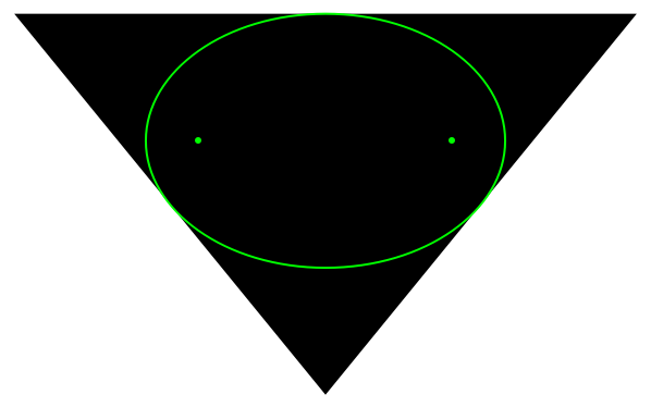 |
Find the roots of a set of points:
| In[4]:= |
| Out[5]= |
By the Lucas–Gauss theorem, the convex hull of the roots is entirely contained by the convex hull of the original points:
| In[6]:= | ![Legended[
Graphics[{FaceForm[], AbsolutePointSize[4], {EdgeForm[ColorData[97, 3]], ColorData[97, 3], ConvexHullMesh[p], Point[p]}, {EdgeForm[ColorData[97, 4]], ColorData[97, 4], ConvexHullMesh[d], Point[d]}}], PointLegend[{ColorData[97, 3], ColorData[97, 4]}, {"original", "derivative"}]]](https://www.wolframcloud.com/obj/resourcesystem/images/699/69956883-05e0-4b7e-be51-fe40ac0c25e3/1955a13985ca19e5.png) |
| Out[7]= | 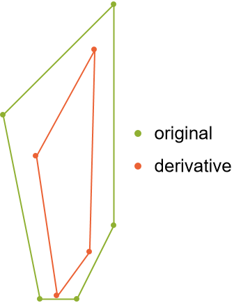 |
| In[8]:= |
| Out[8]= |
The root of two points is the midpoint:
| In[9]:= |
| Out[8]= |
The root of three points is given by the foci of the ellipse tangent to the midpoints of the triangle:
| In[10]:= | ![p3 = RandomReal[{-2, 2}, {3, 2}];
d3 = ResourceFunction["PointsetDerivativeRoots"][p3];
Graphics[{Triangle[p3], Green, ResourceFunction["FociPointEllipse"][
Append[d3, Mean[Take[p3, 2]]]],
Red, Point[d3]}, ImageSize -> Small]](https://www.wolframcloud.com/obj/resourcesystem/images/699/69956883-05e0-4b7e-be51-fe40ac0c25e3/615623502c9f5c21.png) |
| Out[11]= |  |
This is equivalent to the Steiner circumellipse, scaled by a factor of 1/2:
| In[12]:= | ![Graphics[{Triangle[p3], Green, TransformedRegion[ResourceFunction["SteinerCircumellipse"][p3], ScalingTransform[{1/2, 1/2}, Mean[d3]]],
Red, Point[d3]}, ImageSize -> Small]](https://www.wolframcloud.com/obj/resourcesystem/images/699/69956883-05e0-4b7e-be51-fe40ac0c25e3/5c6003d45727cb57.png) |
| Out[13]= | 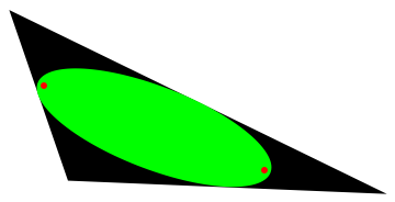 |
Much as in a convex hull, duplicating a point will not affect the result:
| In[14]:= | ![pts = {{Sqrt[6], 1}, {-Sqrt[6], 1}, {0, -2}, {0, -2}};
foci = ResourceFunction["PointsetDerivativeRoots"][pts]](https://www.wolframcloud.com/obj/resourcesystem/images/699/69956883-05e0-4b7e-be51-fe40ac0c25e3/60bee4d85a90fbcc.png) |
| Out[15]= |
Show eleven levels of the Lucas-Gauss theorem:
| In[16]:= | ![p11 = RandomReal[{-2, 2}, {13, 2}];
d11 = NestList[ ResourceFunction["PointsetDerivativeRoots"][#] &, p11,
10];
Graphics[{EdgeForm[Black], White, ConvexHullMesh[#] & /@ d11, Table[{Hue[n/12], Point[d11[[n]]]}, {n, 1, 11}]}, ImageSize -> {400, 300}]](https://www.wolframcloud.com/obj/resourcesystem/images/699/69956883-05e0-4b7e-be51-fe40ac0c25e3/69d86991abd21ec3.png) |
| Out[18]= | 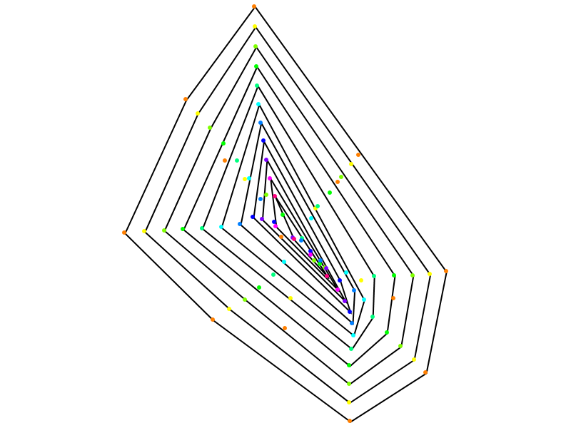 |
This work is licensed under a Creative Commons Attribution 4.0 International License