Wolfram Function Repository
Instant-use add-on functions for the Wolfram Language
Function Repository Resource:
Plots high-dimensional datasets across parallel axes
ResourceFunction["ParallelCoordinatesPlot"][mat] visualizes mat with a parallel coordinates plot. | |
ResourceFunction["ParallelCoordinatesPlot"][mat,cols] labels the plot axes that correspond to data columns with cols. | |
ResourceFunction["ParallelCoordinatesPlot"][mat,cols,ranges] determines the span of each data column in the plot by the two-column matrix ranges. |
| "AxesOrder" | Automatic | order of the axes (data columns) |
| "Colors" | Automatic | colors to be used for multiple data |
| "Direction" | "Horizontal" | direction of the plot |
| "LabelsOffset" | Automatic | offset for the axes labels |
| "PlotAxesGrid" | True | whether to plot the axes grid |
| PlotStyle | Automatic | plot style |
Visualize the rows of a matrix:
| In[1]:= |
|
| Out[2]= |
|
Visualize the rows of matrices in an association:
| In[3]:= |
|
| Out[4]= |
|
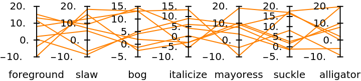
Visualize the rows of a matrix using column names:
| In[5]:= |
![SeedRandom[2]
ResourceFunction["ParallelCoordinatesPlot"][
RandomReal[{-10, 20}, {8, 7}], RandomWord[7], PlotStyle -> Orange]](https://www.wolframcloud.com/obj/resourcesystem/images/22c/22cec55b-ff99-4ff7-87fb-22cb33cc8636/534d1852180440f0.png)
|
| Out[6]= |
|
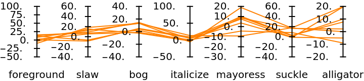
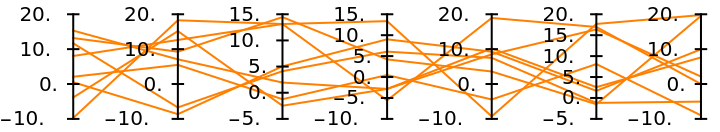
Visualize the rows of a matrix using column names and axes ranges:
| In[7]:= |
![SeedRandom[2]
ResourceFunction["ParallelCoordinatesPlot"][
RandomReal[{-10, 20}, {8, 7}], RandomWord[7], Transpose[{Round@RandomReal[{-30, -10}, 7], Round@RandomReal[{10, 100}, 7]}], PlotStyle -> Orange]](https://www.wolframcloud.com/obj/resourcesystem/images/22c/22cec55b-ff99-4ff7-87fb-22cb33cc8636/188e019f58e81e9e.png)
|
| Out[8]= |
|
Visualize without labels for the data columns' names:
| In[9]:= |
|
| Out[10]= |
|
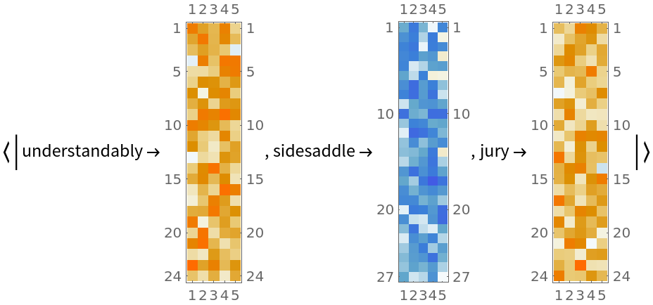
Here is an association of matrices with the same number of columns and different number of rows:
| In[11]:= |
![SeedRandom[7]
aRData = Association@
MapThread[
RandomWord[] -> RandomVariate[
NormalDistribution[#1, Abs[#1]/2], {#2, 5}] &, {{2, -1, 4}, RandomInteger[{20, 30}, 3]}];
MatrixPlot /@ aRData](https://www.wolframcloud.com/obj/resourcesystem/images/22c/22cec55b-ff99-4ff7-87fb-22cb33cc8636/7b58946f790a9772.png)
|
| Out[13]= |
|
| In[14]:= |
|
| Out[14]= |
|
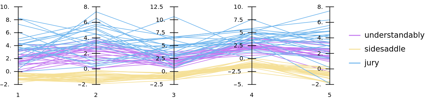
Here we visualize the multidimensional data of each matrix using a (combined) parallel coordinates plot:
| In[15]:= |
|
| Out[15]= |
|
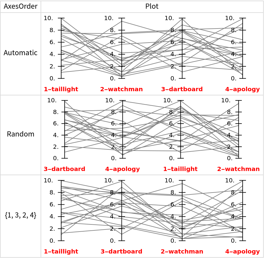
Changing the axes order (the order of the data columns) might produce more informative plots:
| In[16]:= |
![SeedRandom[4]
mat = RandomReal[{0, 10}, {20, 4}];
colNames = Style[#, Red, Bold] & /@ MapIndexed[ToString[#2[[1]]] <> "-" <> #1 &, RandomWord[Length@mat[[1]]]];
Grid[Prepend[
Table[{i, ResourceFunction["ParallelCoordinatesPlot"][mat, colNames, "AxesOrder" -> i, PlotStyle -> Gray, ImageSize -> Medium]}, {i, {Automatic, Random, {1, 3, 2, 4}}}], {"AxesOrder", "Plot"}], Dividers -> All,
FrameStyle -> LightGray]](https://www.wolframcloud.com/obj/resourcesystem/images/22c/22cec55b-ff99-4ff7-87fb-22cb33cc8636/150b0eace6b1663e.png)
|
| Out[9]= |
|
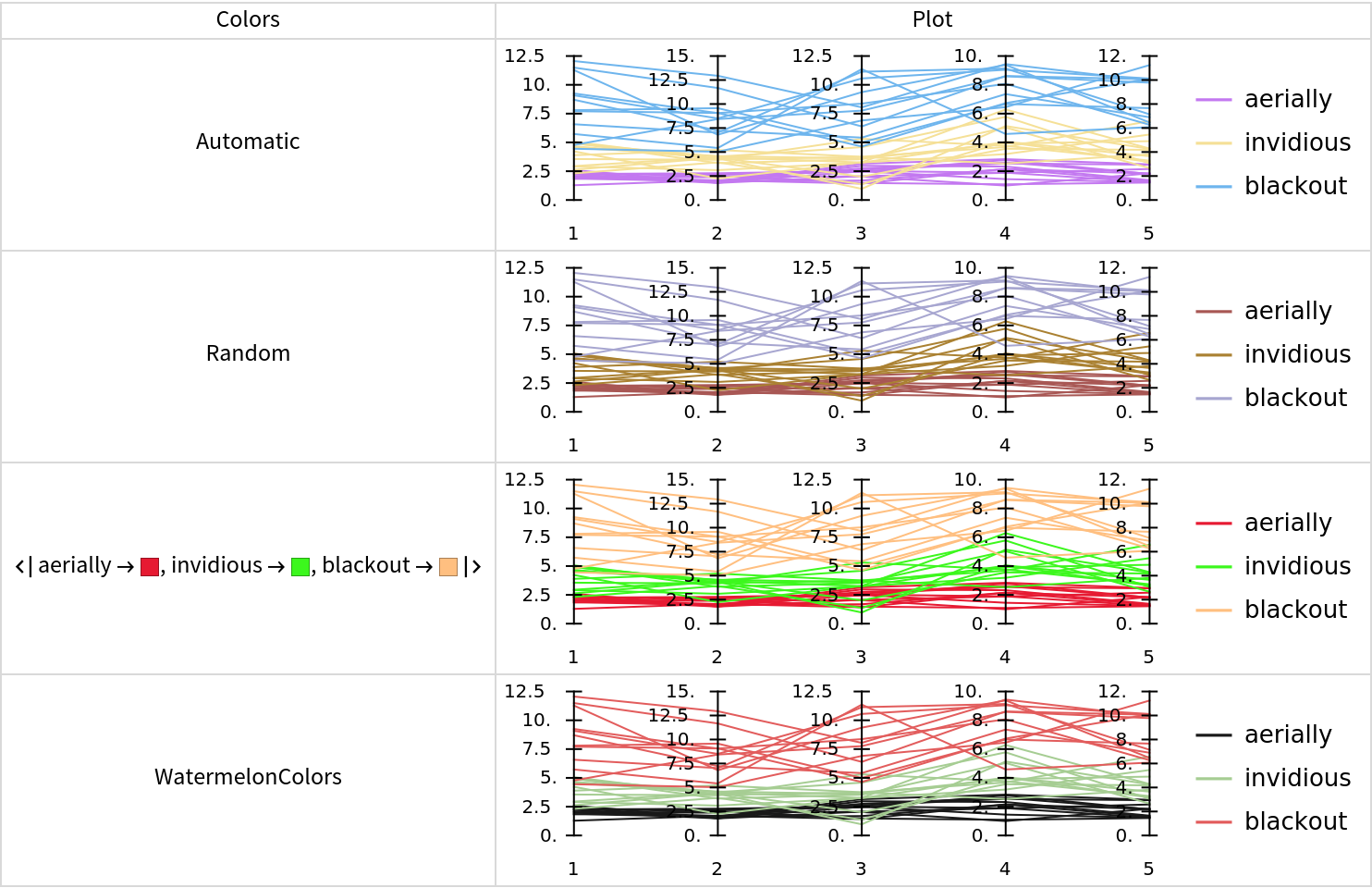
The option "Colors" specifies the coloring of the rows of the different matrices:
| In[17]:= |
![SeedRandom[8]
aMats = Association[
RandomWord[] -> RandomVariate[NormalDistribution[#, #/4], {12, 5}] & /@ {2, 4, 8}];
Grid[Prepend[
Table[{i, ResourceFunction["ParallelCoordinatesPlot"][aMats, "Colors" -> i, ImageSize -> Medium]}, {i, {Automatic, Random, AssociationThread[Keys[aMats], ColorData["BrightBands"] /@ Rescale[Range[Length@aMats]]], "WatermelonColors"}}], {"Colors", "Plot"}], Dividers -> All, FrameStyle -> LightGray]](https://www.wolframcloud.com/obj/resourcesystem/images/22c/22cec55b-ff99-4ff7-87fb-22cb33cc8636/471da53a53ceab3d.png)
|
| Out[7]= |
|
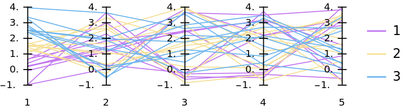
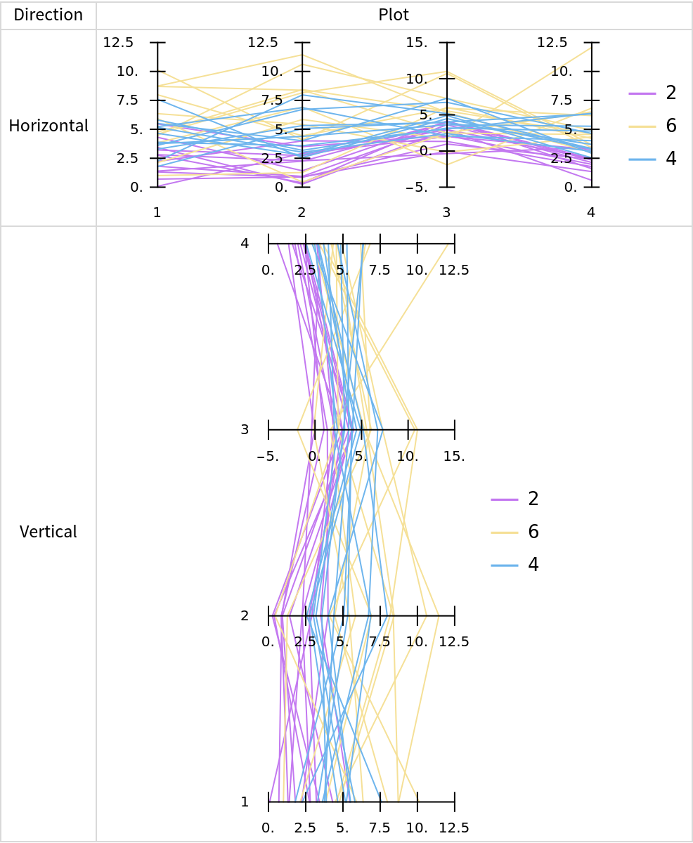
For some data, it is easier to see patterns through vertical parallel coordinates plots:
| In[18]:= |
![SeedRandom[5]
aMats = Association[# -> RandomVariate[NormalDistribution[#, #/2], {12, 4}] & /@ {2, 6, 4}];
Grid[Prepend[
Table[{i, ResourceFunction["ParallelCoordinatesPlot"][aMats, "Direction" -> i, ImageSize -> Medium]}, {i, {"Horizontal", "Vertical"}}], {"Direction", "Plot"}], Dividers -> All, FrameStyle -> LightGray]](https://www.wolframcloud.com/obj/resourcesystem/images/22c/22cec55b-ff99-4ff7-87fb-22cb33cc8636/06ce0c50864837e5.png)
|
| Out[7]= |
|
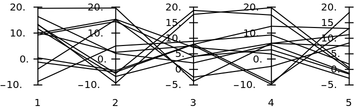
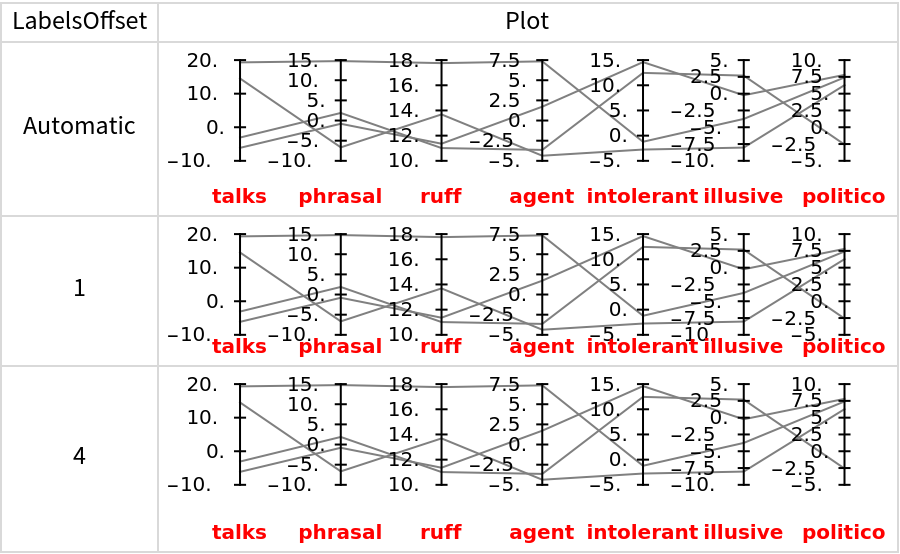
The option "LabelsOffset" allows tweaking of the axes labels' locations:
| In[19]:= |
![SeedRandom[1]
mat = RandomReal[{-10, 20}, {4, 7}];
colNames = Style[#, Red, Bold] & /@ RandomWord[Length@mat[[1]]];
Grid[Prepend[
Table[{i, ResourceFunction["ParallelCoordinatesPlot"][mat, colNames, "LabelsOffset" -> i, PlotStyle -> Gray, ImageSize -> Medium]}, {i, {Automatic, 1, 4}}], {"LabelsOffset", "Plot"}], Dividers -> All, FrameStyle -> LightGray]](https://www.wolframcloud.com/obj/resourcesystem/images/22c/22cec55b-ff99-4ff7-87fb-22cb33cc8636/13213f4dc705de4f.png)
|
| Out[9]= |
|
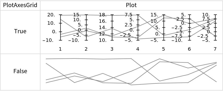
If the value of the option "PlotAxesGrid" is False, then no axes grid is plotted:
| In[20]:= |
![SeedRandom[1]
mat = RandomReal[{-10, 20}, {4, 7}];
Grid[Prepend[
Table[{i, ResourceFunction["ParallelCoordinatesPlot"][mat, "PlotAxesGrid" -> i, PlotStyle -> Gray, ImageSize -> Medium]}, {i, {True, False}}], {"PlotAxesGrid", "Plot"}], Dividers -> All, FrameStyle -> LightGray]](https://www.wolframcloud.com/obj/resourcesystem/images/22c/22cec55b-ff99-4ff7-87fb-22cb33cc8636/35bd14b9526dfaa1.png)
|
| Out[7]= |
|
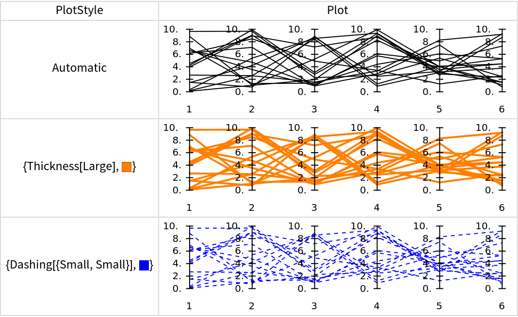
The option PlotStyle can be used to specify how the lines corresponding to the data elements are drawn:
| In[21]:= |
![SeedRandom[9]
mat = RandomReal[{0, 10}, {16, 6}];
Grid[Prepend[
Table[{i, ResourceFunction["ParallelCoordinatesPlot"][mat, PlotStyle -> i, ImageSize -> Medium]}, {i, {Automatic, {Thick, Orange}, {Dashed, Blue}}}], {PlotStyle, "Plot"}], Dividers -> All, FrameStyle -> LightGray]](https://www.wolframcloud.com/obj/resourcesystem/images/22c/22cec55b-ff99-4ff7-87fb-22cb33cc8636/167c8f56fddf260b.png)
|
| Out[7]= |
|
Get the "FisherIris" dataset:
| In[22]:= |
|
| Out[23]= |
|
Split the iris data into groups defined by the species column (which is the last column):
| In[24]:= |
|
| Out[25]= |
|
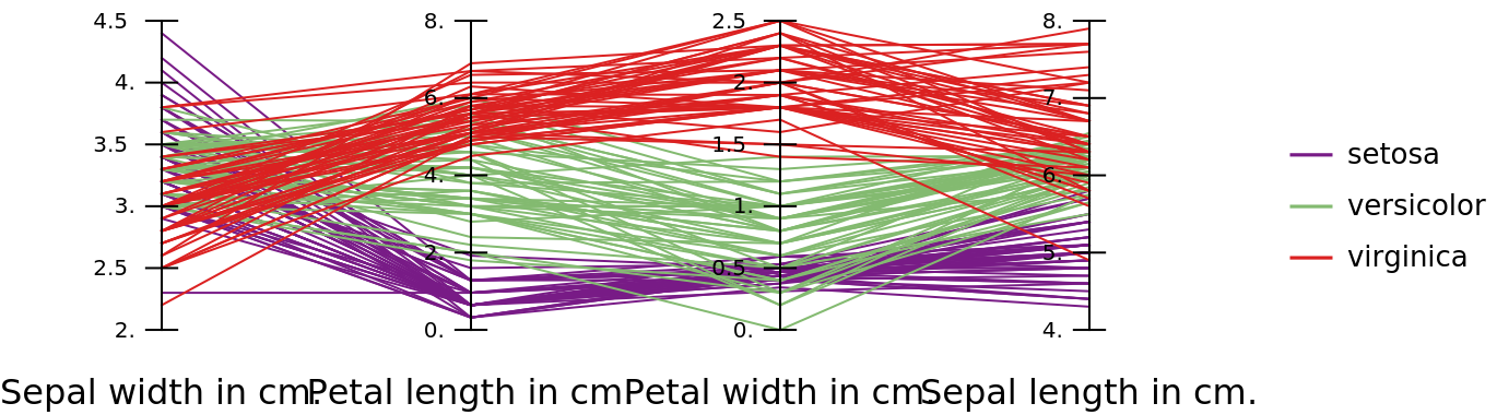
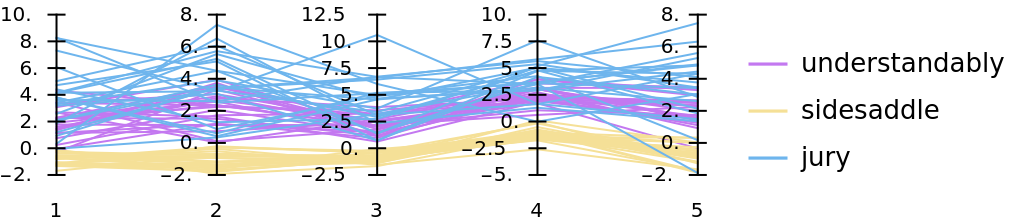
Use ParallelCoordinatesPlot to visualize the differences between subsets of data:
| In[26]:= |
![ResourceFunction["ParallelCoordinatesPlot"][aData, Style[#, FontSize -> 16] & /@ Most[colNames], "Colors" -> "Rainbow", "AxesOrder" -> Random, Direction -> "Horizontal", ImageSize -> Large]](https://www.wolframcloud.com/obj/resourcesystem/images/22c/22cec55b-ff99-4ff7-87fb-22cb33cc8636/29e93b2995f5a5ae.png)
|
| Out[26]= |
|
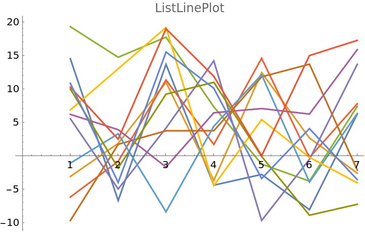
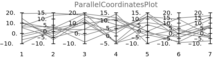
ParallelCoordinatesPlot can be seen as an extension of ListLinePlot:
| In[27]:= |
![SeedRandom[1]
mat = RandomReal[{-10, 20}, {12, 7}];
ListLinePlot[mat, PlotLabel -> "ListLinePlot"]](https://www.wolframcloud.com/obj/resourcesystem/images/22c/22cec55b-ff99-4ff7-87fb-22cb33cc8636/44f1beeb5457cdc4.png)
|
| Out[29]= |
|
| In[30]:= |
|
| Out[30]= |
|
If the first argument is an association of matrices, then the third argument (for the axes ranges) is always taken to be Automatic:
| In[31]:= |
|
| Out[31]= |
|
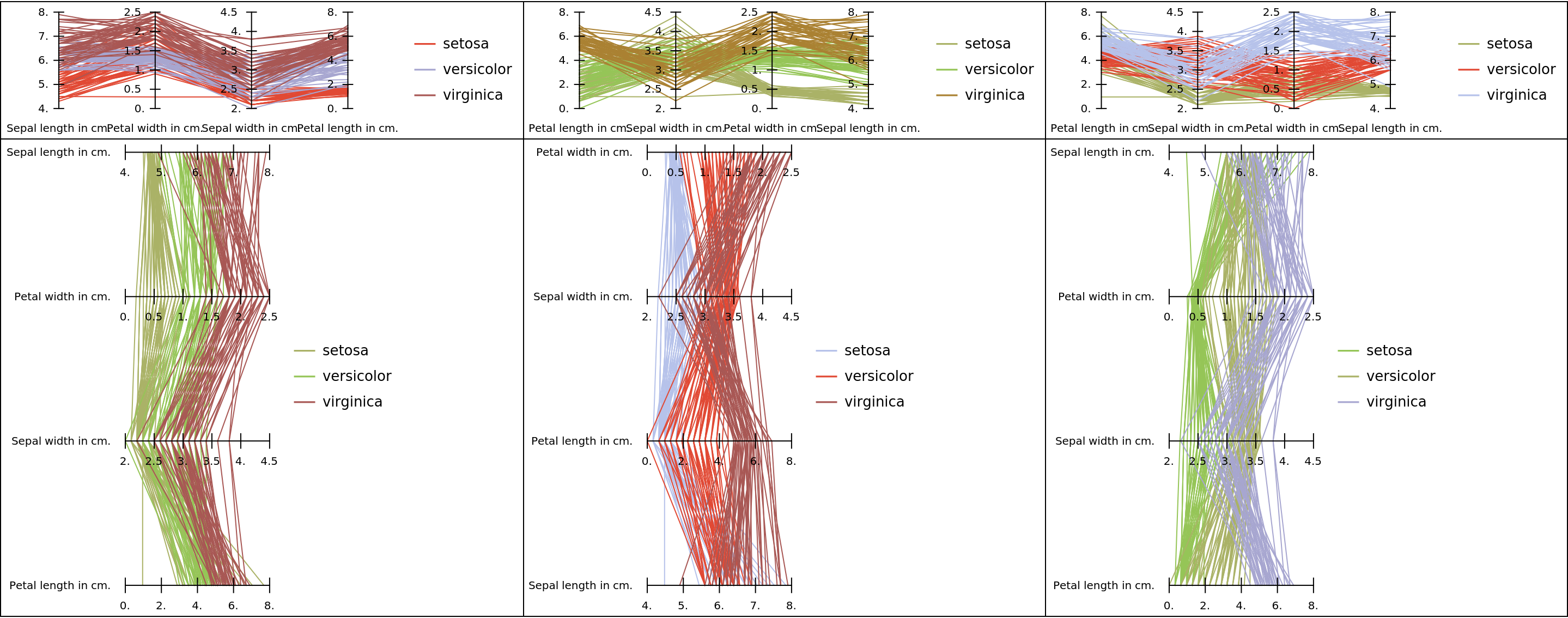
Make a grid of parallel coordinates plots using the "FisherIris" dataset:
| In[32]:= |
![SeedRandom[12];
data = ExampleData[{"Statistics", "FisherIris"}];
colNames = ExampleData[{"Statistics", "FisherIris"}, "ColumnDescriptions"];
aData = GroupBy[data, #[[-1]] &, #[[All, 1 ;; -2]] &];
grs = Table[
ResourceFunction["ParallelCoordinatesPlot"][aData, Most[colNames], "Colors" -> Random, "AxesOrder" -> Random, Direction -> dir, ImageSize -> Medium], {dir, {"Horizontal", "Vertical"}}, {m, 3}];
Grid[grs, Alignment -> Left, Dividers -> All]](https://www.wolframcloud.com/obj/resourcesystem/images/22c/22cec55b-ff99-4ff7-87fb-22cb33cc8636/357f1d79b7864c41.png)
|
| Out[5]= |
|
This work is licensed under a Creative Commons Attribution 4.0 International License