Wolfram Function Repository
Instant-use add-on functions for the Wolfram Language
Function Repository Resource:
Evaluate the divided difference of a finite orthogonal polynomial series
ResourceFunction["OrthogonalPolynomialDividedDifference"][cof,poly,x,y] evaluates the divided difference |
| "ChebyshevFirst" | Chebyshev polynomial of the first kind ChebyshevT[i,x] |
| "ChebyshevSecond" | Chebyshev polynomial of the second kind ChebyshevU[i,x] |
| "Hermite" | Hermite polynomial HermiteH[i,x] |
| "Laguerre" | Laguerre polynomial LaguerreL[i,x] |
| "Legendre" | Legendre polynomial LegendreP[i,x] |
| {"Gegenbauer",m} | Gegenbauer polynomial GegenbauerC[i,m,x] |
| {"Laguerre",a} | associated Laguerre polynomial LaguerreL[i,a,x] |
| {"Jacobi",a,b} | Jacobi polynomial JacobiP[i,a,b,x] |
Divided difference of a Laguerre series:
| In[1]:= |
|
| Out[1]= |
|
Compare with an explicit evaluation using the resource function OrthogonalPolynomialSum:
| In[2]:= |
![With[{c = {1/2, -1/4, 1/8, -1/16}, x = 4/3, y = 1}, (ResourceFunction["OrthogonalPolynomialSum"][c, "Laguerre", x] - ResourceFunction["OrthogonalPolynomialSum"][c, "Laguerre", y])/(x - y)]](https://www.wolframcloud.com/obj/resourcesystem/images/81f/81f2b102-edc9-4085-9303-d4346f85d74b/71877d9a9fd75e41.png)
|
| Out[2]= |
|
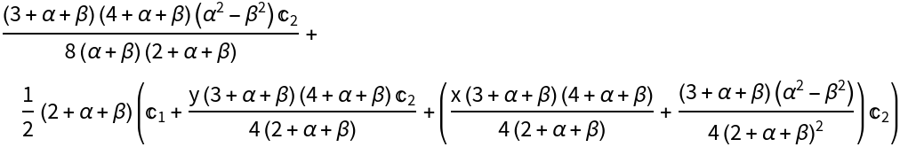
Divided difference of a Jacobi series with symbolic coefficients, parameters and arguments:
| In[3]:= |
|
| Out[3]= |
|
An equivalent specification:
| In[4]:= |
|
| Out[4]= |

|
Directly evaluating the divided difference using the resource function OrthogonalPolynomialSum gives a result that is not very accurate:
| In[5]:= |
![With[{c = {1/2, -1/4, 1/8, -1/16}, \[CurlyEpsilon] = N[3*^-8, 20]}, (ResourceFunction["OrthogonalPolynomialSum"][
c, {"Laguerre", -1/2}, 5 + \[CurlyEpsilon]] - ResourceFunction["OrthogonalPolynomialSum"][c, {"Laguerre", -1/2},
5 - \[CurlyEpsilon]])/((5 + \[CurlyEpsilon]) - (5 - \
\[CurlyEpsilon]))]](https://www.wolframcloud.com/obj/resourcesystem/images/81f/81f2b102-edc9-4085-9303-d4346f85d74b/72dd222f25633976.png)
|
| Out[5]= |
|
OrthogonalPolynomialDividedDifference gives a more accurate result:
| In[6]:= |
![With[{c = {1/2, -1/4, 1/8, -1/16}, \[CurlyEpsilon] = N[3*^-8, 20]}, ResourceFunction["OrthogonalPolynomialDividedDifference"][
c, {"Laguerre", -1/2}, 5 - \[CurlyEpsilon], 5 + \[CurlyEpsilon]]]](https://www.wolframcloud.com/obj/resourcesystem/images/81f/81f2b102-edc9-4085-9303-d4346f85d74b/277acccfd7ac5e2d.png)
|
| Out[6]= |
|
Evaluate the q-derivative of a Chebyshev series:
| In[7]:= |
|
| Out[7]= |
|
In the limit q→1, the q-derivative reduces to the derivative:
| In[8]:= |
|
| Out[8]= |
|
| In[9]:= |
|
| Out[9]= |
|
OrthogonalPolynomialDividedDifference is symmetric in the arguments x and y:
| In[10]:= |
![ResourceFunction["OrthogonalPolynomialDividedDifference"][
Array[C, 4, 0], "Legendre", x, y] == ResourceFunction["OrthogonalPolynomialDividedDifference"][
Array[C, 4, 0], "Legendre", y, x] // Simplify](https://www.wolframcloud.com/obj/resourcesystem/images/81f/81f2b102-edc9-4085-9303-d4346f85d74b/14112a4b68820a0c.png)
|
| Out[10]= |
|
If x=y, the result of OrthogonalPolynomialDividedDifference is equal to the derivative of the orthogonal polynomial series, evaluated at x:
| In[11]:= |
![ResourceFunction["OrthogonalPolynomialDividedDifference"][
Array[C, 4, 0], "Legendre", x, x] == (D[
ResourceFunction["OrthogonalPolynomialSum"][Array[C, 4, 0], "Legendre", t], t] /. t -> x) // Simplify](https://www.wolframcloud.com/obj/resourcesystem/images/81f/81f2b102-edc9-4085-9303-d4346f85d74b/2ec3600e423de2e7.png)
|
| Out[11]= |
|
This work is licensed under a Creative Commons Attribution 4.0 International License