Wolfram Function Repository
Instant-use add-on functions for the Wolfram Language
Function Repository Resource:
Use graph algorithms from the Python package NetworkX without any Python programming
ResourceFunction["NetworkXObject"][] returns a configured PythonObject for the Python package NetworkX in a new Python session. | |
ResourceFunction["NetworkXObject"][session] uses the specified running ExternalSessionObject session. | |
ResourceFunction["NetworkXObject"][…,"func"[args,opts]] executes the function func with the specified arguments and options. |
Create a NetworkX object:
| In[1]:= |
| Out[1]= |
Construct an undirected graph from an edge list:
| In[2]:= |
| In[3]:= |
| Out[3]= |
Import the Python object as a Graph:
| In[4]:= |
| Out[4]= |  |
The imported graph is a standard Wolfram Language object:
| In[5]:= |
| Out[5]= |
| In[6]:= |
| Out[6]= | 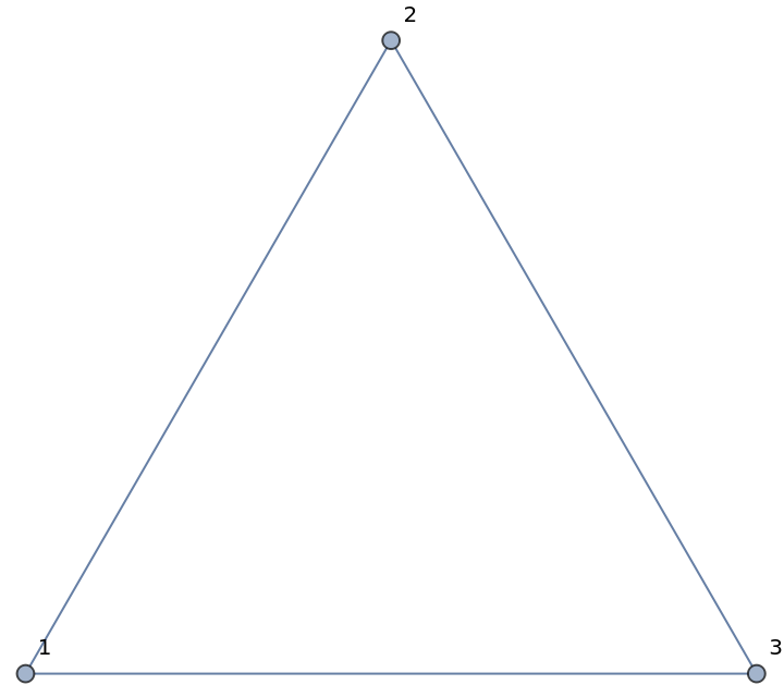 |
Get a directed graph:
| In[7]:= |
| Out[7]= |
| In[8]:= |
| Out[8]= | 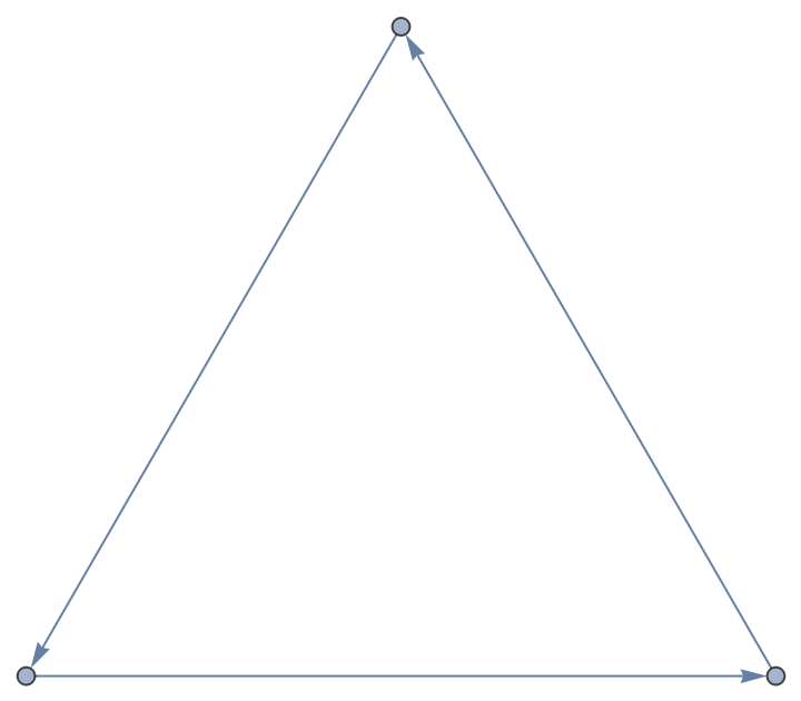 |
| In[9]:= |
| Out[9]= |
Clean up the Python session:
| In[10]:= |
An undirected graph supporting multiple edges between vertices:
| In[11]:= |
| Out[11]= |
| In[12]:= |
| In[13]:= |
| Out[13]= |
| In[14]:= |
| Out[14]= | 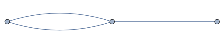 |
| In[15]:= |
| Out[15]= |
A directed multigraph:
| In[16]:= |
| Out[16]= |
| In[17]:= |
| Out[17]= | 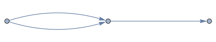 |
| In[18]:= |
| Out[18]= |
| In[19]:= |
Create an empty graph:
| In[20]:= |
| Out[20]= |
| In[21]:= |
| Out[21]= |
Nodes and edges of the graph are given as continuously updated NodeView and EdgeView objects:
| In[22]:= |
| Out[22]= | 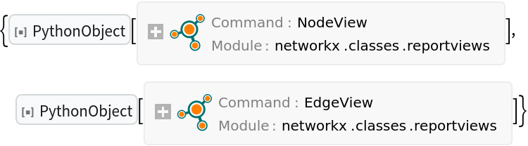 |
| In[23]:= |
| Out[23]= |
Add one node at a time:
| In[24]:= |
Examine nodes:
| In[25]:= |
| Out[25]= |
| In[26]:= |
| Out[26]= |
Remove a node:
| In[27]:= |
| In[28]:= |
| Out[28]= |
Add nodes from a list:
| In[29]:= |
| In[30]:= |
| Out[30]= |
Remove several nodes:
| In[31]:= |
| In[32]:= |
| Out[32]= |
| In[33]:= |
| In[34]:= |
| Out[34]= |
| In[35]:= |
| Out[35]= |
Add nodes along with node attributes specified as an Association:
| In[36]:= |
| In[37]:= |
| Out[37]= |
Retrieve the specified node attribute:
| In[38]:= |
| Out[38]= |
Check the attributes of the imported graph:
| In[39]:= |
| Out[39]= |  |
| In[40]:= |
| Out[40]= |
| In[41]:= |
| Out[41]= |
| In[42]:= |
Create a new graph:
| In[43]:= |
| Out[43]= |
| In[44]:= |
| Out[44]= |
To add a node attribute after a node is created, get a reference to the Python dictionary of node attributes:
| In[45]:= |
| In[46]:= |
| Out[46]= |  |
Adding a key→value pair to the dictionary adds an attribute to the graph:
| In[47]:= |
| Out[47]= |
| In[48]:= |
| Out[48]= |
| In[49]:= |
Create a new graph:
| In[50]:= |
| Out[50]= |
| In[51]:= |
| Out[51]= |
Grow the graph by adding one edge at a time:
| In[52]:= |
| In[53]:= |
| Out[53]= |
Add a list of edges:
| In[54]:= |
Add a list of edges with attributes:
| In[55]:= |
| In[56]:= |
| Out[56]= |
Check the attributes in the imported graph:
| In[57]:= |
| Out[57]= | 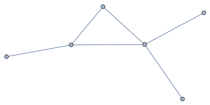 |
| In[58]:= |
| Out[58]= |
| In[59]:= |
| Out[59]= |
To add an edge attribute after an edge is created, assign a key→value pair to the dictionary of edge attributes:
| In[60]:= |
| Out[60]= |  |
| In[61]:= |
| Out[61]= |
Confirm the assignment for the edge 12:
| In[62]:= |
| Out[62]= |
Remove a single edge:
| In[63]:= |
| In[64]:= |
| Out[64]= |
Remove several edges:
| In[65]:= |
| In[66]:= |
| Out[66]= |
| In[67]:= |
Create a new empty graph:
| In[68]:= |
| Out[68]= |
Incorporate nodes from one graph into another:
| In[69]:= |
| Out[69]= | 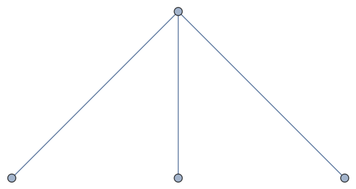 |
| In[70]:= |
| Out[70]= |
| In[71]:= |
| In[72]:= |
| Out[72]= |
| In[73]:= |
| Out[73]= |  |
| In[74]:= |
Create a new empty graph:
| In[75]:= |
| Out[75]= |
Use one graph as a node in another:
| In[76]:= |
| Out[76]= |
| In[77]:= |
| Out[77]= |
| In[78]:= |
| In[79]:= |
| Out[79]= |
| In[80]:= |
| Out[80]= | 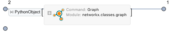 |
| In[81]:= |
Create a new empty graph:
| In[82]:= |
| Out[82]= |
| In[83]:= |
| Out[83]= |
Add a node "spam":
| In[84]:= |
Add four nodes "s", "p", "a", "m":
| In[85]:= |
| In[86]:= |
| Out[86]= |
| In[87]:= |
Create a new empty graph:
| In[88]:= |
| Out[88]= |
| In[89]:= |
| Out[89]= |
Incorporate edges from one graph into another:
| In[90]:= |
| Out[90]= |  |
| In[91]:= |
| Out[91]= |
| In[92]:= |
| In[93]:= |
| Out[93]= |
| In[94]:= |
| Out[94]= | 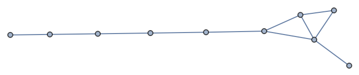 |
| In[95]:= |
Create a new multi-digraph graph:
| In[96]:= |
| Out[96]= |
| In[97]:= |
| Out[97]= |
Add edges with weights:
| In[98]:= |
| In[99]:= |
| Out[99]= |
| In[100]:= |
| Out[100]= |
| In[101]:= |
Create a new multi-digraph:
| In[102]:= |
| Out[102]= |
Count nodes and edges in a graph:
| In[103]:= |
| Out[103]= |
| In[104]:= |
| Out[104]= | 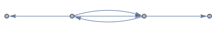 |
| In[105]:= |
| Out[105]= |
| In[106]:= |
| Out[106]= |
| In[107]:= |
Create a new multi-digraph:
| In[108]:= |
| Out[108]= |
| In[109]:= |
| Out[109]= |
| In[110]:= |
| Out[110]= | 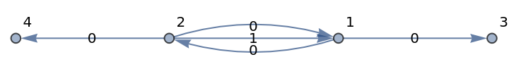 |
Test whether a node is in the graph:
| In[111]:= |
| Out[111]= | 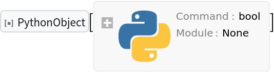 |
| In[112]:= |
| Out[112]= |
Test if an edge is in the graph:
| In[113]:= |
| Out[113]= |
Test if an edge with a specific tag is in the graph:
| In[114]:= |
| Out[114]= |
Use the DirectedEdge wrapper in the edge specification:
| In[115]:= |
| Out[115]= |
| In[116]:= |
Create a new multi-digraph:
| In[117]:= |
| Out[117]= |
| In[118]:= |
| Out[118]= |
Get an Association of neighbors (adjacencies) as a property of the graph:
| In[119]:= |
| Out[119]= |
| In[120]:= |
| Out[120]= |
Alternatively, use the "Adjacency" method to get a list of tuples rather than an Association:
| In[121]:= |
| Out[121]= |  |
| In[122]:= |
| Out[122]= |
| In[123]:= |
Create a new multi-digraph:
| In[124]:= |
| Out[124]= |
| In[125]:= |
| Out[125]= |
Get an object containing vertex degrees for all vertices in the graph:
| In[126]:= |
| Out[126]= |
| In[127]:= |
| Out[127]= |
The degree of a specific vertex:
| In[128]:= |
| Out[128]= |
| In[129]:= |
Create a new multi-digraph:
| In[130]:= |
| Out[130]= |
| In[131]:= |
| Out[131]= |
Get a list of neighbors for a node:
| In[132]:= |
| Out[132]= |  |
| In[133]:= |
| Out[133]= |
Or equivalently, for a directed graph:
| In[134]:= |
| Out[134]= |
Predecessors of a node of a directed graph:
| In[135]:= |
| Out[135]= |
| In[136]:= |
Create a new graph:
| In[137]:= |
| Out[137]= |
| In[138]:= |
| Out[138]= |
Use the special attribute "weight" to create a waited graph:
| In[139]:= |
Alternatively, use the AddWeightedEdgesFrom method:
| In[140]:= |
Compute the weighted adjacency matrix on the Python side:
| In[141]:= |
| Out[141]= |  |
Import the matrix as SparseArray:
| In[142]:= |
| Out[142]= |
| In[143]:= |
| Out[143]= |
The imported graph is weighted too:
| In[144]:= |
| Out[144]= |  |
| In[145]:= |
| Out[145]= |
| In[146]:= |
| Out[146]= |
| In[147]:= |
| Out[147]= |
Compare with the adjacency matrix computed in Python:
| In[148]:= |
| Out[148]= |
| In[149]:= |
Create a new NetworkX object:
| In[150]:= |
| Out[150]= |
| In[151]:= |
Undirected and directed graphs with self-loops and a single edge between nodes:
| In[152]:= |
| Out[152]= |  |
| In[153]:= |
| Out[153]= | 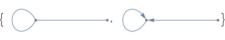 |
| In[154]:= |
| Out[154]= |
Undirected and directed graphs possibly with parallel edges between nodes:
| In[155]:= |
| Out[155]= | 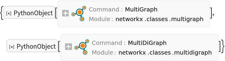 |
| In[156]:= |
| Out[156]= | 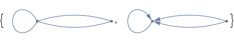 |
| In[157]:= |
| Out[157]= |
Edges in imported multigraphs are tagged:
| In[158]:= |
| Out[158]= |
| In[159]:= |
Build a graph incrementally:
| In[160]:= |
| Out[160]= |
| In[161]:= |
| In[162]:= |
| In[163]:= |
| Out[163]= |  |
| In[164]:= |
Create from an edge list:
| In[165]:= |
| Out[165]= |
Alternatively, use the edge list in the form returned by EdgeList:
| In[166]:= |
| Out[166]= |
| In[167]:= |
| Out[167]= |
| In[168]:= |
Form an Association mapping nodes to neighbors:
| In[169]:= |
| Out[169]= |
| In[170]:= |
| Out[170]= |  |
| In[171]:= |
Form a general Wolfram Language Graph:
| In[172]:= |
| Out[172]= |  |
| In[173]:= |
| Out[173]= | 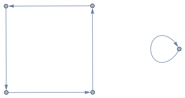 |
From a sparse matrix graph:
| In[174]:= |
| Out[174]= |
| In[175]:= |
| Out[175]= | 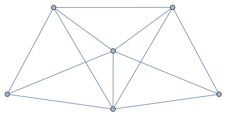 |
| In[176]:= |
| Out[176]= |  |
| In[177]:= |
From a weighted Graph object:
| In[178]:= |
| In[179]:= |
| Out[179]= | 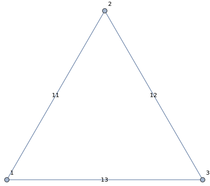 |
| In[180]:= |
| Out[180]= |
| In[181]:= |
| Out[181]= |  |
| In[182]:= |
From an edge-capacity and vertex-capacity Graph object:
| In[183]:= |
| Out[183]= |  |
Send the graph through NetworkX:
| In[184]:= |
| Out[184]= |
| In[185]:= |
| Out[185]= |  |
The capacity is preserved as an annotation:
| In[186]:= |
| Out[186]= |
| In[187]:= |
| Out[187]= |
| In[188]:= |
From a multigraph:
| In[189]:= |
| In[190]:= |
| Out[190]= |
| In[191]:= |
| Out[191]= |  |
| In[192]:= |
From another NetworkX graph:
| In[193]:= |
| Out[193]= |  |
| In[194]:= |
| Out[194]= |  |
| In[195]:= |
Form a 2D NumPy array:
| In[196]:= |
| Out[196]= |
Create a graph and import it:
| In[197]:= | ![nx = ResourceFunction["NetworkXObject"][];
np = ResourceFunction["PythonObject"][
nx["Session"], <|"Command" -> "``", "TemplateArguments" -> {arr}|>]](https://www.wolframcloud.com/obj/resourcesystem/images/15d/15de1605-6c74-4421-8560-82793e1100aa/5f9bc78b305638ac.png) |
| Out[197]= | 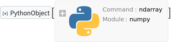 |
| In[198]:= |
| Out[198]= | 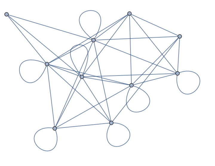 |
The same NumPy array can be supplied implicitly, as long as the array is in the form of NumericArray:
| In[199]:= |
| Out[199]= |  |
| In[200]:= |
Create a graph from a SciPy sparse matrix:
| In[201]:= |
| Out[201]= |  |
| In[202]:= |
| Out[202]= |
| In[203]:= |
| Out[203]= |  |
| In[204]:= |
| Out[204]= | 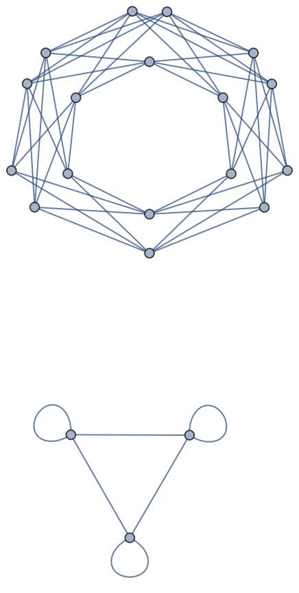 |
Or from a SciPy sparse array:
| In[205]:= |
| Out[205]= |  |
| In[206]:= |
| Out[206]= |  |
| In[207]:= |
Create a graph directly from a SparseArray object:
| In[208]:= | ![s = SparseArray[{Band[{2, 1}] -> 1, Band[{3, 1}] -> 1}, {10, 10}];
nx = ResourceFunction["NetworkXObject"][];
Normal[nx["Graph"[s]]]](https://www.wolframcloud.com/obj/resourcesystem/images/15d/15de1605-6c74-4421-8560-82793e1100aa/61199b7dac2171f0.png) |
| Out[208]= |  |
| In[209]:= |
Create a data frame from a pandas object:
| In[210]:= | ![nx = ResourceFunction["NetworkXObject"][];
pd = ResourceFunction["PandasObject"][nx["Session"]];
df = pd["DataFrame"[{{1, 1}, {2, 1}}]]](https://www.wolframcloud.com/obj/resourcesystem/images/15d/15de1605-6c74-4421-8560-82793e1100aa/317ba91b0988dd6f.png) |
| Out[208]= |
Create a graph:
| In[211]:= |
| Out[211]= |
Or use the FromPandasAdjacency function:
| In[212]:= |
| Out[212]= |
| In[213]:= |
| Out[213]= | 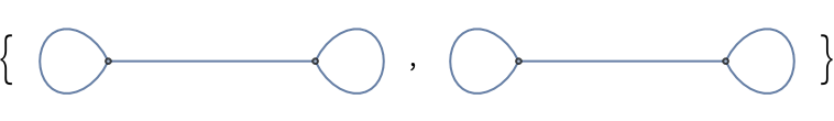 |
| In[214]:= |
Create a data frame representing a pandas edge list:
| In[215]:= | ![nx = ResourceFunction["NetworkXObject"][];
pd = ResourceFunction["PandasObject"][nx["Session"]];
df = pd["DataFrame"[<|"source" -> {0, 1, 2, 0}, "target" -> {2, 2, 3, 2}, "my_edge_key" -> {"A", "B", "C", "D"}, "weight" -> {3, 4, 5, 6}, "color" -> {"red", "blue", "blue", "blue"}|>]]](https://www.wolframcloud.com/obj/resourcesystem/images/15d/15de1605-6c74-4421-8560-82793e1100aa/7b98d5976bb9af36.png) |
| Out[208]= |
Convert to a graph:
| In[216]:= | ![g = nx["FromPandasEdgeList"[
df,
"EdgeKey" -> "my_edge_key",
"EdgeAttr" -> {"weight", "color"},
"CreateUsing" -> nx["MultiGraph"[]]
]
]](https://www.wolframcloud.com/obj/resourcesystem/images/15d/15de1605-6c74-4421-8560-82793e1100aa/080cd958aa1201e9.png) |
| Out[216]= |
See the Graph:
| In[217]:= |
| Out[217]= |  |
See the edge list and weights:
| In[218]:= |
| Out[218]= |  |
Compare with a dataset:
| In[219]:= |
| Out[219]= | 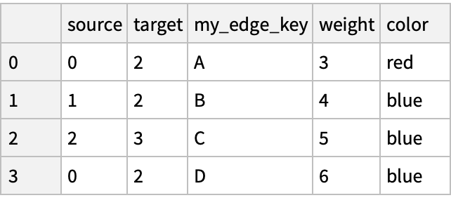 |
| In[220]:= |
Explore the variety of ways to generate graphs:
| In[221]:= |
| In[222]:= |
| Out[222]= | 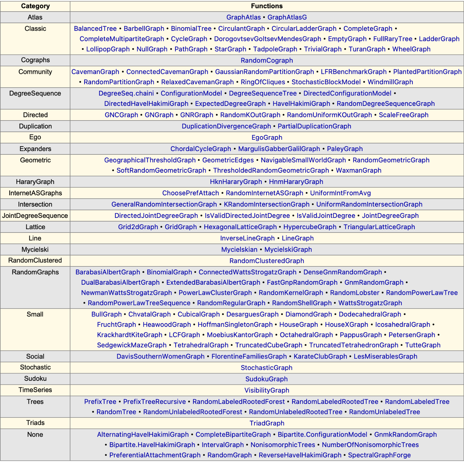 |
| In[223]:= |
Create the first few scale-free pseudo-fractal graphs using the Dorogovtsev-Goltsev-Mendes algorithm:
| In[224]:= |
| Out[224]= | 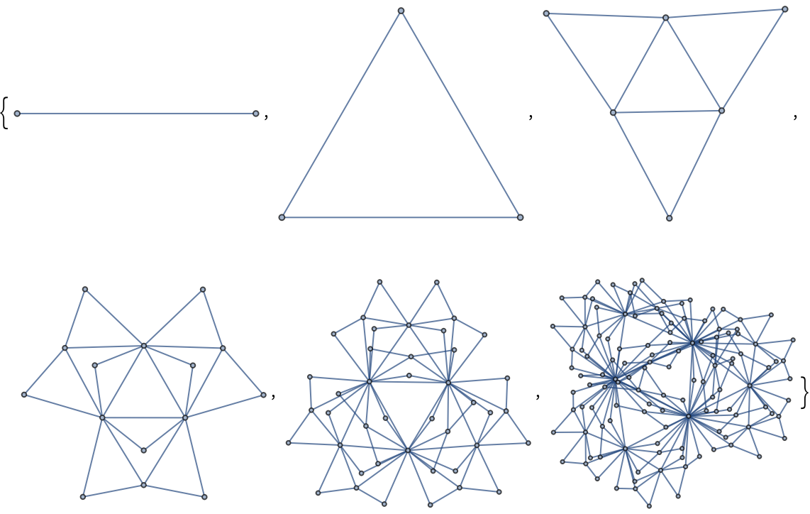 |
| In[225]:= |
A few Newman–Watts–Strogatz small-world graphs:
| In[226]:= |
| Out[226]= | 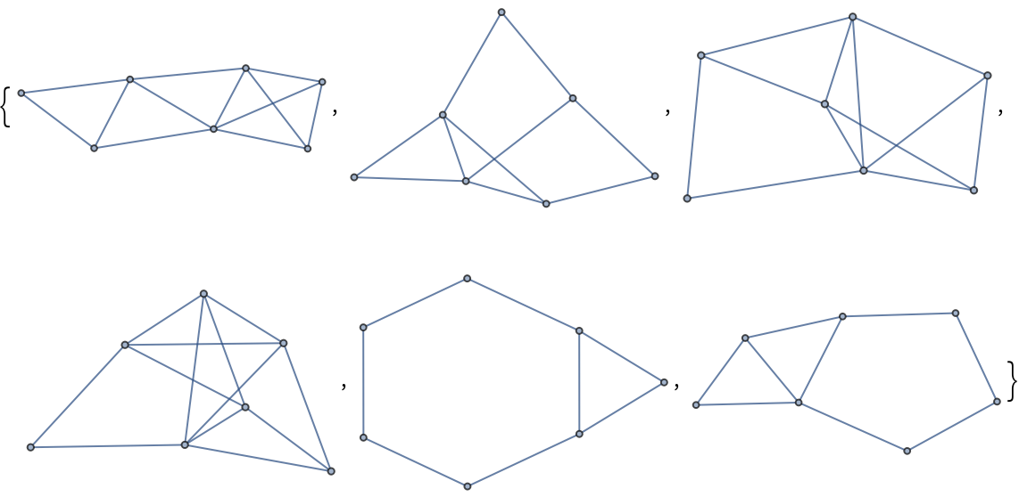 |
| In[227]:= |
The specified graph from the Graph Atlas:
| In[228]:= |
| Out[228]= | 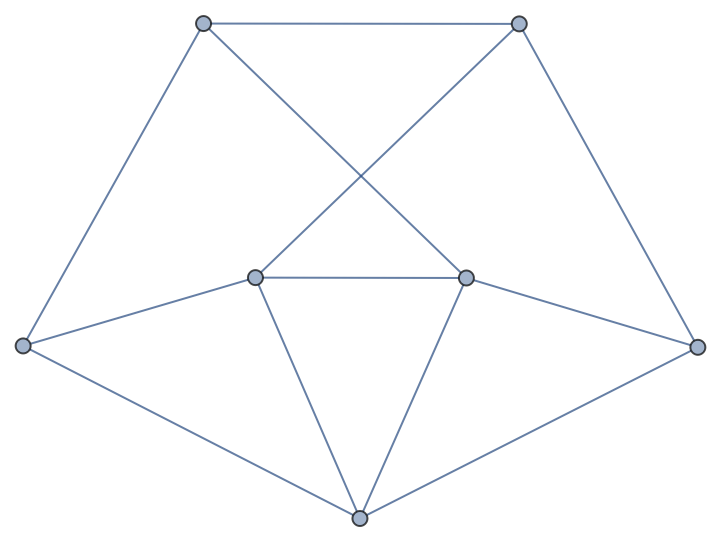 |
| In[229]:= |
A Zachary’s Karate Club graph:
| In[230]:= |
| Out[230]= | 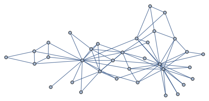 |
The same graph in the Wolfram Language (but note that NetworkX version is kept on the Python side):
| In[231]:= |
| Out[231]= | 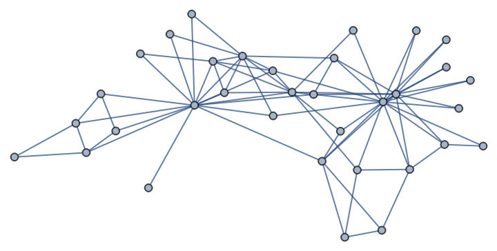 |
Create a series of random Spectral Graph Forge (SGF) graphs resembling the global properties of the previous graph:
| In[232]:= |
| Out[232]= | 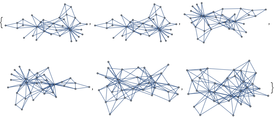 |
| In[233]:= |
A bipartite random graph with the first n nodes in the first bipartite set and the remaining m nodes in the second:
| In[234]:= | ![n = 5; m = 10;
nx = ResourceFunction["NetworkXObject"][];
nx["RandomGraph"[n, m, .75, "Seed" -> 1]] // Normal](https://www.wolframcloud.com/obj/resourcesystem/images/15d/15de1605-6c74-4421-8560-82793e1100aa/34479c91e8a09362.png) |
| Out[234]= | 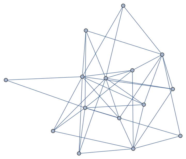 |
Show the bipartite partition of the graph:
| In[235]:= |
| Out[235]= | 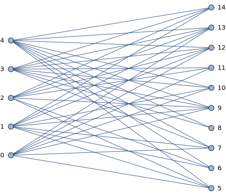 |
| In[236]:= |
A random partition graph:
| In[237]:= |
| Out[237]= | 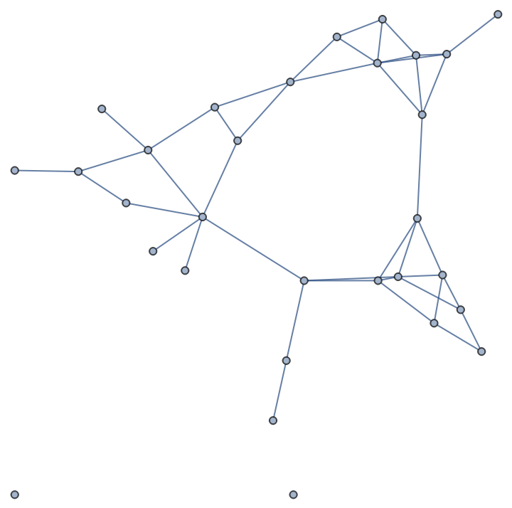 |
| In[238]:= |
| Out[238]= |
| In[239]:= |
A Gaussian random partition graph:
| In[240]:= |
| Out[240]= | 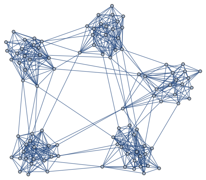 |
| In[241]:= |
| Out[241]= |  |
Highlight the partitions:
| In[242]:= |
| Out[242]= | 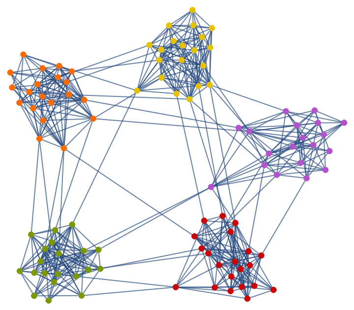 |
Explore functional interface to graph methods and assorted graph utilities:
| In[243]:= |
| Out[243]= | 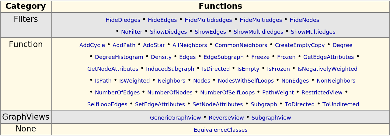 |
| In[244]:= |
Add a star to a graph, with the first node in the middle of the star and the other nodes connected to it:
| In[245]:= | ![nx = ResourceFunction["NetworkXObject"][];
g = nx["Graph"[]];
nx["AddStar"[g, {0, 1, 2, 3}]]](https://www.wolframcloud.com/obj/resourcesystem/images/15d/15de1605-6c74-4421-8560-82793e1100aa/30e26c55383d5b1e.png) |
| In[246]:= |
| Out[246]= | 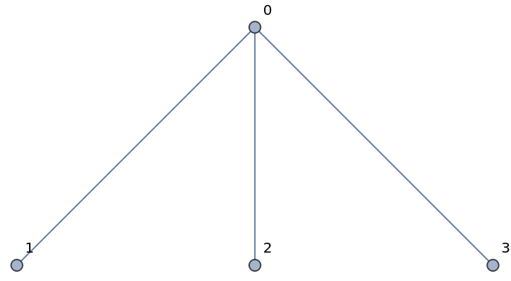 |
Add another star, with weighted edges:
| In[247]:= |
| In[248]:= |
| Out[248]= |  |
| In[249]:= |
Explore available graph-theoretic algorithms:
| In[250]:= |
| Out[250]= | 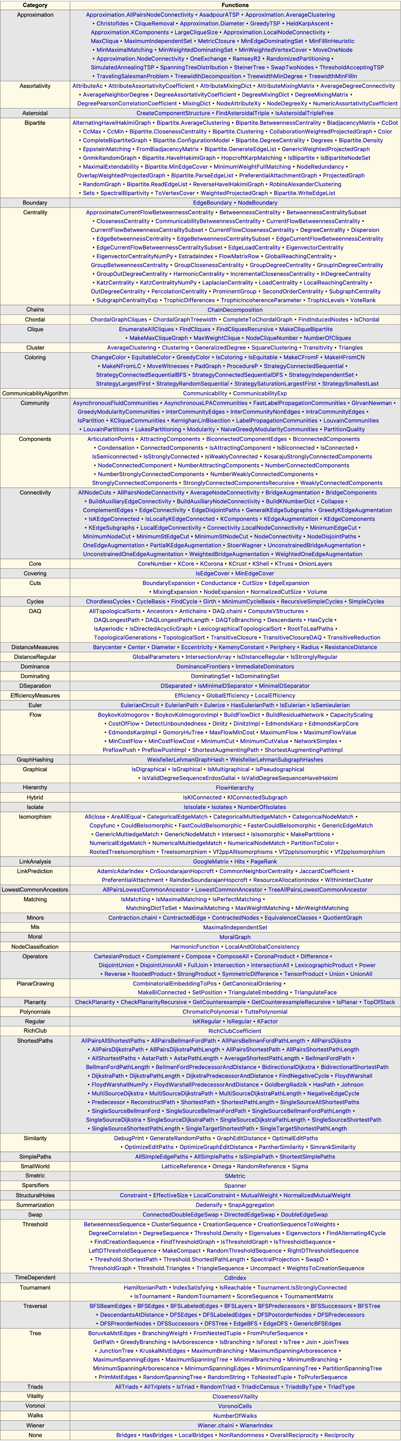 |
| In[251]:= |
Create a random bipartite graph with n nodes in the first bipartite set and compute the biadjacency matrix of the graph:
| In[252]:= | ![nx = ResourceFunction["NetworkXObject"][];
n = 5;
g = nx["RandomGraph"[n, 10, .75, "Seed" -> 1]]](https://www.wolframcloud.com/obj/resourcesystem/images/15d/15de1605-6c74-4421-8560-82793e1100aa/4aec1480cb3ea0ab.png) |
| Out[252]= |
| In[253]:= |
| Out[253]= |  |
| In[254]:= |
| Out[254]= |  |
Despite being smaller, the biadjacency matrix fully describes the graph:
| In[255]:= |
| Out[255]= |  |
| In[256]:= |
| Out[256]= |
| In[257]:= |
Compute the clustering coefficient for nodes of a complete graph:
| In[258]:= |
| Out[258]= |  |
| In[259]:= |
| Out[259]= |
The clustering coefficient for the specified nodes:
| In[260]:= |
| Out[260]= |
For a single node:
| In[261]:= |
| Out[261]= |
| In[262]:= |
Compute the average clustering coefficient for nodes of a random Erdős-Rényi (binomial) graph:
| In[263]:= |
| Out[263]= |  |
| In[264]:= |
| Out[264]= |
| In[265]:= |
Find the dominating set of a random geometric graph:
| In[266]:= |
| Out[266]= | 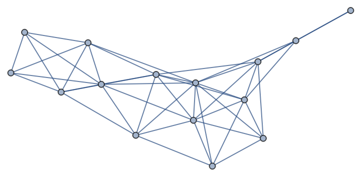 |
| In[267]:= |
| Out[267]= |
Confirm that the set of vertices form a dominating set:
| In[268]:= |
| Out[268]= | 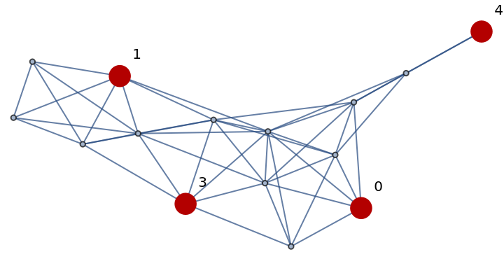 |
| In[269]:= |
| Out[269]= |
| In[270]:= |
Define a hidden Markov model (HMM) graph with five states and observation nodes:
| In[271]:= |
| Out[271]= |
| In[272]:= |
Check if states/observation nodes before "S3" are d-separated from the states/observations after "S3":
| In[273]:= |
| In[274]:= |
| In[275]:= |
| In[276]:= |
| Out[276]= |
| In[277]:= |
| Out[277]= | 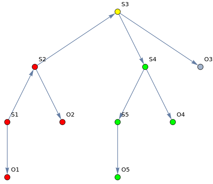 |
| In[278]:= |
Create an undirected moralized graph of given a directed graph:
| In[279]:= |
| Out[279]= |
| In[280]:= |
| Out[280]= |
Display the graphs:
| In[281]:= |
| Out[281]= | 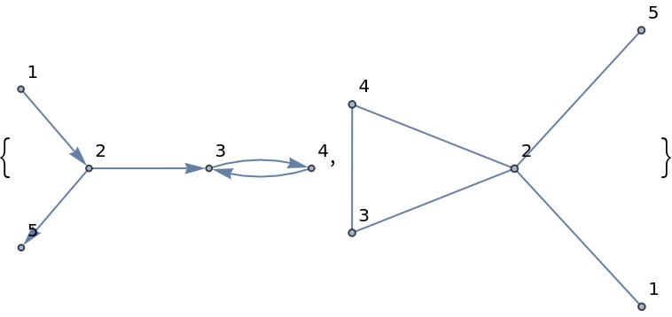 |
The added edge between unconnected parents that have a common child:
| In[282]:= |
| Out[282]= |
| In[283]:= |
Functions for drawing graphs include interfaces to Python packages PyGraphviz, PyDot, PyLab:
| In[284]:= |
| Out[284]= | 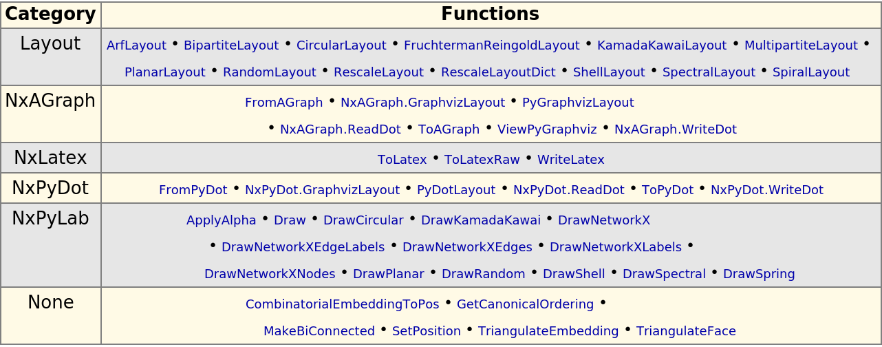 |
| In[285]:= |
Create a Matplotlib object to draw a graph on the Python side:
| In[286]:= |
| Out[286]= |
Prepare a subplot object to plot a graph:
| In[287]:= |
| Out[287]= |
Create and plot the graph in Python:
| In[288]:= |
| Out[288]= |
| In[289]:= |
| Out[289]= |
| In[290]:= |
Import the graph image:
| In[291]:= |
| Out[291]= | 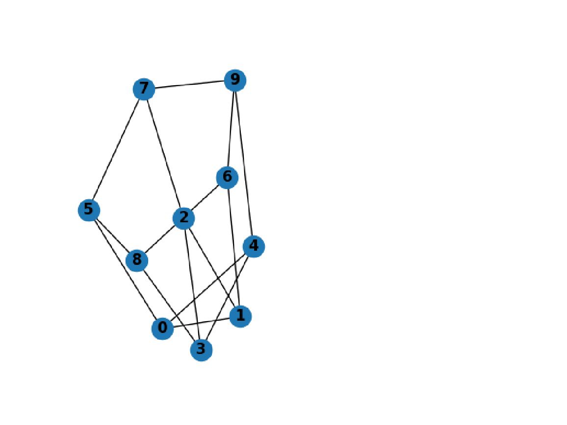 |
Prepare another subplot and draw the graph with shell layout:
| In[292]:= |
| Out[292]= |
| In[293]:= | ![nx["DrawShell"[g, "nlist" -> {Range[5, 9], Range[0, 4]}, "WithLabels" -> True, "FontWeight" -> "bold"]]](https://www.wolframcloud.com/obj/resourcesystem/images/15d/15de1605-6c74-4421-8560-82793e1100aa/7e4a03a71f123234.png) |
Import the combined image:
| In[294]:= |
| Out[294]= | 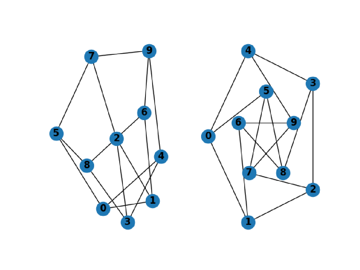 |
| In[295]:= |
Display a table graph-theoretical functions for linear algebra:
| In[296]:= |
| Out[296]= | 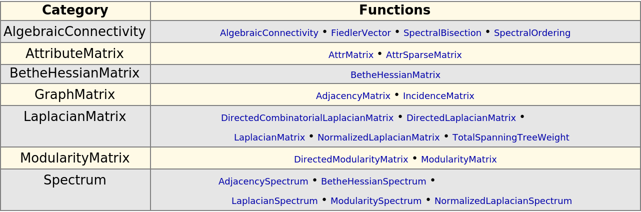 |
| In[297]:= |
Construct a simple graph with given degree sequence using the Havel-Hakimi algorithm:
| In[298]:= |
| Out[298]= |  |
The Bethe Hessian matrix of the graph:
| In[299]:= |
| Out[299]= |  |
| In[300]:= |
| Out[300]= |  |
| In[301]:= |
Display a table of functions that import, export and process data in common graph formats:
| In[302]:= |
| Out[302]= | 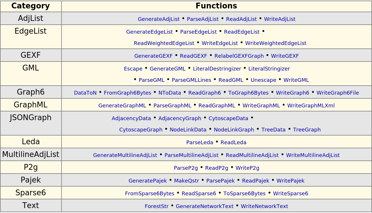 |
| In[303]:= |
Create a graph:
| In[304]:= |
| Out[341]= | 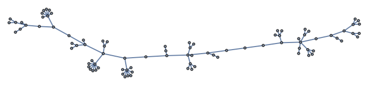 |
Export the graph in the Graph6 format:
| In[342]:= |
| In[343]:= |
Import the file in Python:
| In[344]:= |
| Out[344]= |
| In[345]:= |
| Out[345]= |  |
Import the file in the Wolfram Language:
| In[346]:= |
| Out[346]= |  |
| In[347]:= |
Explore the available graph utilities:
| In[348]:= |
| Out[348]= | 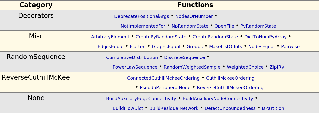 |
Utilities called by graph constructors that can also be called directly (and functions for converting back):
| In[349]:= |
| Out[349]= |  |
| In[350]:= |
Create an edge list using "Pairwise":
| In[351]:= |
| Out[64]= | 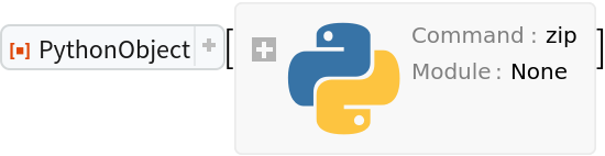 |
Partition creates an analogous list:
| In[352]:= |
| Out[352]= |
Create graphs from each to show the equivalence:
| In[353]:= |
| Out[353]= | 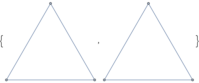 |
| In[354]:= |
Convert a graph to a SciPy sparse array:
| In[355]:= |
| Out[355]= |
| In[356]:= |
| Out[356]= | 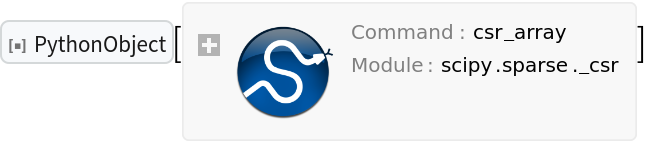 |
Import the matrix:
| In[357]:= |
| Out[357]= |
| In[358]:= |
Control the type of returned object in graph constructors using the option CreateUsing:
| In[359]:= |
| Out[359]= |  |
| In[360]:= |
| Out[360]= | 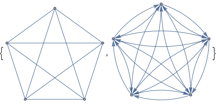 |
| In[361]:= |
Functions, such as "RelabelNodes", that have the option "Copy" allow you to modify the input graph object in-place:
| In[362]:= |
| Out[362]= |  |
By default, "RelabelNodes" returns a modified graph keeping the original intact:
| In[363]:= |
| Out[363]= |
Define the remapping:
| In[364]:= |
| Out[364]= |
| In[365]:= |
| Out[365]= |
Show the original and remapped vertex names:
| In[366]:= |
| Out[366]= |
Use "Copy"→False to modify the input graph in-place:
| In[367]:= |
| Out[367]= |
The graph g has changed:
| In[368]:= |
| Out[368]= | 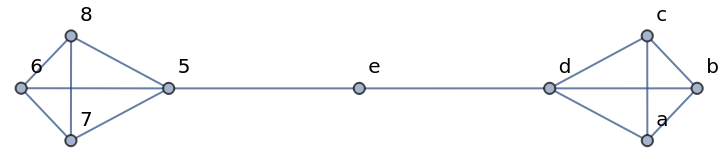 |
| In[369]:= |
The option "Seed" seeds the random number generator in functions that use randomness to generate, draw and compute properties or manipulate graphs.
Create a line graph:
| In[370]:= |
| Out[370]= |
Define a function that computes random coordinates of a graph, passing options to RandomLayout:
| In[371]:= |
Without a seed, executing the function twice produces different sets of random coordinates:
| In[372]:= |
| Out[372]= | 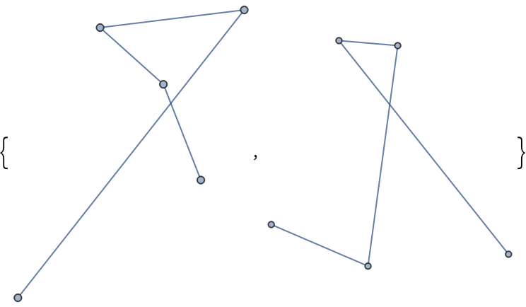 |
Use the option "Seed" to create a reproducible random layout:
| In[373]:= |
| Out[373]= | 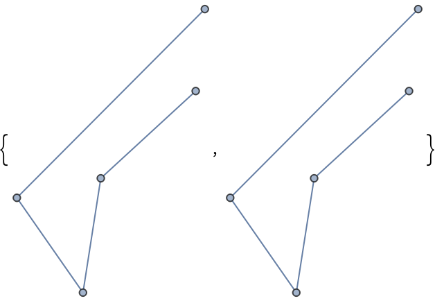 |
| In[374]:= |
Employ algorithms that might not yet be implemented in the Wolfram Language; for instance, find an approximate solution to the asymmetric traveling salesman problem using the algorithm developed by Asadpour et al.
Create a weighted directed graph:
| In[375]:= | ![nx = ResourceFunction["NetworkXObject"][];
CompleteGraph[3, DirectedEdges -> True, EdgeWeight -> {1 \[DirectedEdge] 2 -> 2, 2 \[DirectedEdge] 3 -> 2, 3 \[DirectedEdge] 1 -> 2, 1 \[DirectedEdge] 3 -> 1, 3 \[DirectedEdge] 2 -> 1, 2 \[DirectedEdge] 1 -> 1}, VertexLabels -> Automatic, EdgeLabels -> "EdgeWeight"]](https://www.wolframcloud.com/obj/resourcesystem/images/15d/15de1605-6c74-4421-8560-82793e1100aa/5b14a8e1bf1cdd4b.png) |
| Out[375]= | 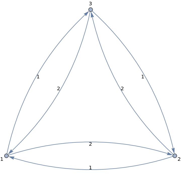 |
Import the graph in Python:
| In[376]:= |
| Out[376]= |
Find the shortest cycle starting and ending at vertex 1:
| In[377]:= |
| Out[377]= |
| In[378]:= |
Create a graph using a constructor that might not yet be implemented in the Wolfram Language, such as a directed graph constructor for the growing network with redirection (the GNR model):
| In[379]:= |
| Out[379]= | 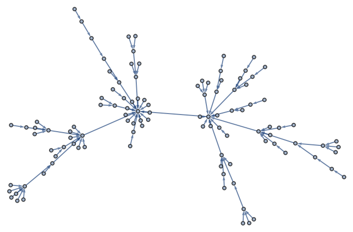 |
| In[380]:= |
Visualize data and draw conclusions from a pandas DataFrame object.
Create a small group of participants:
| In[381]:= | ![n = 20;
SeedRandom[10];
names = ResourceFunction["RandomPetName"][n]](https://www.wolframcloud.com/obj/resourcesystem/images/15d/15de1605-6c74-4421-8560-82793e1100aa/309552405a42729a.png) |
| Out[380]= |
Simulate a table exported from a JIRA bug database:
| In[382]:= |
| In[383]:= |
| Out[383]= |
Create a pandas "DataFrame" object for the database:
| In[384]:= | ![session = StartExternalSession["Python"];
pd = ResourceFunction["PandasObject"][session];
df = pd["DataFrame"[db]]](https://www.wolframcloud.com/obj/resourcesystem/images/15d/15de1605-6c74-4421-8560-82793e1100aa/6cc92cd204cd9416.png) |
| Out[384]= |
| In[385]:= |
| Out[385]= | 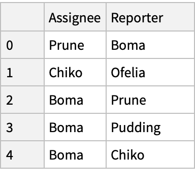 |
Construct a graph of the database:
| In[386]:= |
| Out[386]= |
| In[387]:= |
| Out[387]= |
Team members Boma and Pudding are apparently in the center of action:
| In[388]:= |
| Out[388]= | 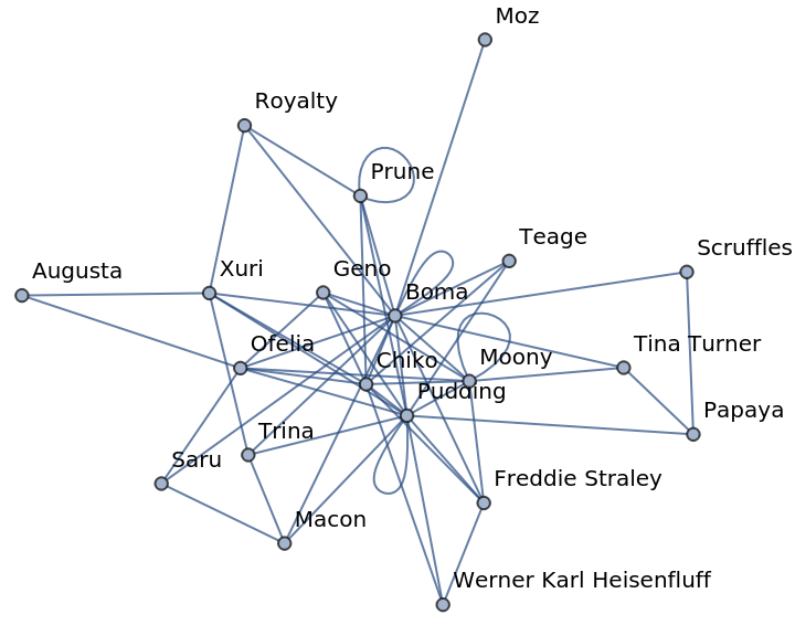 |
Extract all connections represented by edges of the graph:
| In[389]:= |
| Out[389]= |  |
Create a table of participants sorted by activity:
| In[390]:= |
| In[391]:= |
| Out[391]= |  |
| In[392]:= |
NetworkXObject[…] gives the same result as the resource function PythonObject with a special configuration:
| In[393]:= |
| Out[393]= |
| In[394]:= |
| Out[394]= |
| In[395]:= |
Get information on a NetworkX object:
| In[396]:= |
| Out[396]= |
| In[397]:= |
| Out[397]= |
Open the user guide in your default web browser:
| In[398]:= |
| In[399]:= |
Some of the functions and classes available in the NetworkX module:
| In[400]:= |
| Out[400]= |
| In[401]:= |
| Out[401]= |
| In[402]:= |
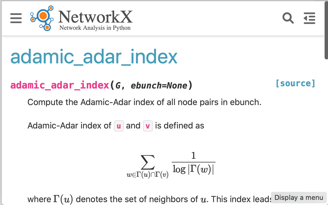
Information on a function:
| In[403]:= |
| Out[403]= |  |
Web documentation of a function:
| In[404]:= |
| In[405]:= |
Functions similar to the given one; click the function name to go to the web documentation:
| In[406]:= |
| Out[406]= |
| In[407]:= |
| Out[407]= | 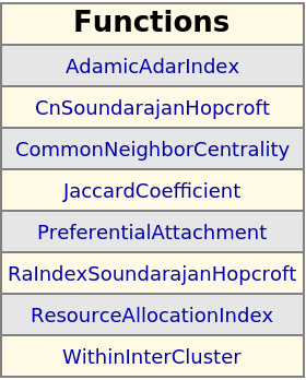 |
| In[408]:= |
Aliases defined for a function or class:
| In[409]:= |
| Out[409]= |
| In[410]:= |
| Out[410]= |
| In[411]:= |
NetworkX Graph objects are analogous to Graph, but keep the objects on the Python side:
| In[412]:= |
| Out[412]= | 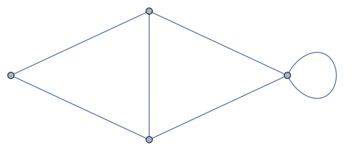 |
| In[413]:= |
| Out[413]= |
Similarly, many graph properties and functions closely correspond to Wolfram Language functions:
| In[414]:= |
| Out[414]= |
| In[415]:= |
| Out[415]= |
| In[416]:= |
Functions of the same name might be defined in different modules:
| In[417]:= |
| Out[417]= |
| In[418]:= |
| In[419]:= |
| Out[419]= |  |
Functions defined for both general and bipartite graphs:
| In[420]:= |
| Out[420]= |  |
| In[421]:= |
Define a bipartite graph in the Wolfram Language and NetworkX:
| In[422]:= |
| Out[422]= | 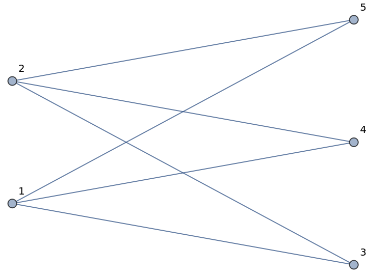 |
| In[423]:= |
| Out[423]= |
The general function "ClosenessCentrality" function can be accessed by an unqualified name, returning the same values as the corresponding Wolfram Language function ClosenessCentrality:
| In[424]:= |
| Out[424]= |
| In[425]:= |
| Out[425]= |
Use a qualified name to access the bipartite version of the function:
| In[426]:= |
| Out[426]= |
| In[427]:= |
NetworkX uses zero-based indexes, while the Wolfram Language Graph uses one-based node indexes:
| In[428]:= |
| Out[428]= |
| In[429]:= |
| Out[429]= |
See the vertex indexing from NetworkX:
| In[430]:= |
| Out[430]= |
Compare with the default indexing in Graph:
| In[431]:= |
| Out[431]= |
Use "RelabelNodes" to index the nodes differently:
| In[432]:= |
| Out[432]= |
Now the indices are identical:
| In[433]:= |
| Out[433]= |
| In[434]:= |
When constructing graphs from Graph, NetworkXObject may not pass all annotations:
| In[435]:= | ![g = PathGraph[Range[3], AnnotationRules -> {1 -> {VertexLabels -> "hello"}, 2 -> {VertexLabels -> "there"}}]](https://www.wolframcloud.com/obj/resourcesystem/images/15d/15de1605-6c74-4421-8560-82793e1100aa/47e5f68d59513526.png) |
| Out[435]= |
| In[436]:= |
| Out[436]= |
Use "SetNodeAttributes" to pass the annotations:
| In[437]:= |
| Out[437]= |
| In[438]:= |
| In[439]:= |
| Out[439]= |
| In[440]:= |
NetworkXObject choses the type of edges in graph constructors based on the graph type, effectively discarding the DirectedEdge and UndirectedEdge wrappers:
| In[441]:= |
| Out[441]= |
| In[442]:= |
| Out[442]= |
Similarly, the wrappers are discarded in all other functions:
| In[443]:= |
| Out[443]= |
| In[444]:= |
An attempt to call a function by an unqualified name might fail if the function is defined in multiple contexts:
| In[445]:= |
| Out[445]= |  |
Use a qualified name to call the bipartite version of the function:
| In[446]:= |
| Out[446]= |
| In[447]:= |
| Out[447]= | 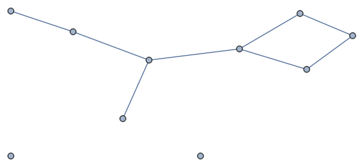 |
Use an unqualified name to call the general function:
| In[448]:= |
| Out[448]= |
| In[449]:= |
| Out[449]= | 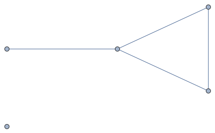 |
| In[450]:= |
Wolfram Language 12.3 (May 2021) or above
The documentation created with:
| In[1]:= |
Loading/caching some parts of the NetworkX package may take time, as seen by the "Amending…" temporary print. Until the resource function PythonObject amends the cache automatically, you can do it manually at any time after one or more of such long operations:
| In[2]:= |
As mentioned in Possible Issues, NetworkXObject currently simply discards the DirectedEdge and UndirectedEdge wrappers, the support for which is added merely as convenience, to facilitate, e.g., shipping the result of EdgeList[] to the nx["Graph"[…] constructor. If we want to be more robust (or more pedantic), we can add a form of type checking down the road.
Random graphs and some of the algorithms from the NetworkX package will be conveniently available using the NetworkXLink paclet when it is published in the Wolfram Language Paclet Repository.
This work is licensed under a Creative Commons Attribution 4.0 International License