Basic Examples (2)
Construct a Matplotlib object:
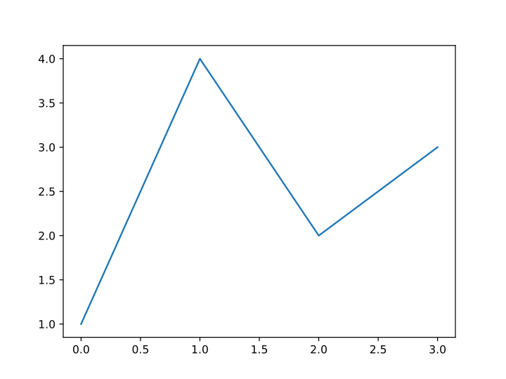
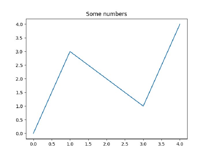
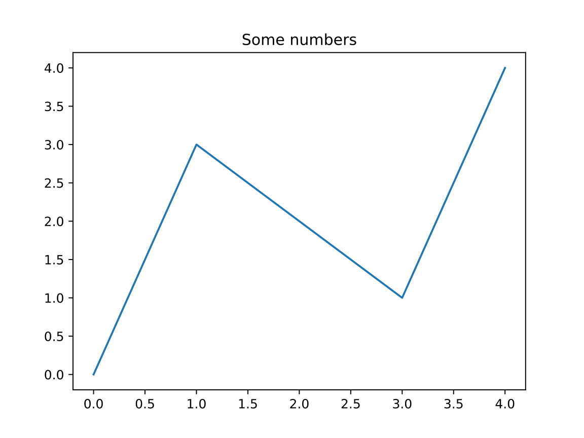
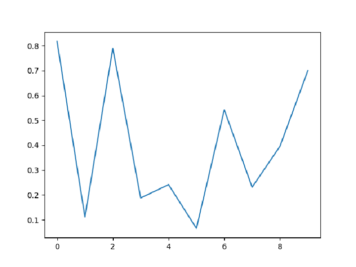
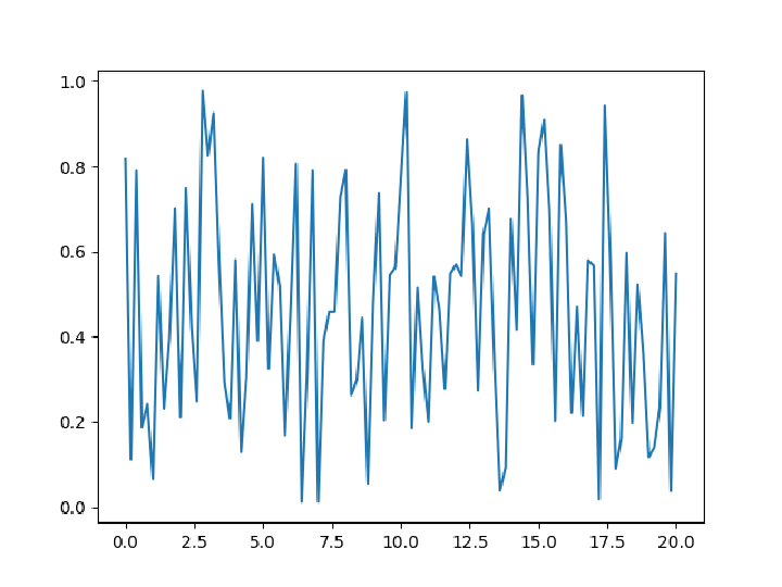
Create a Python object representing a plot of some numbers:
Add a plot label to the object:
Show the plot as an image in the default raster format:
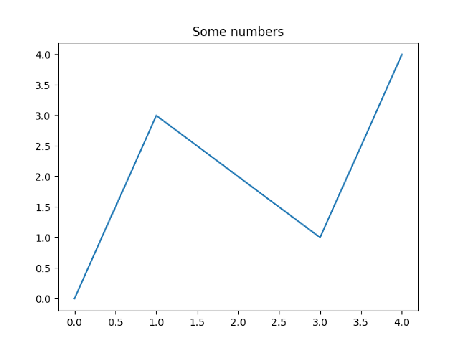
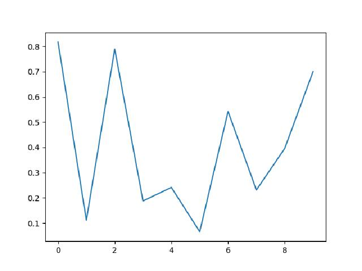
Show the plot as vector graphics:
Save the plot from Python in a temporary directory, without bringing the image to your Wolfram Language session:
Import the file:
Export as a vector graphics:
Import the file:
Clean up by deleting the temporary files and killing the Python session:
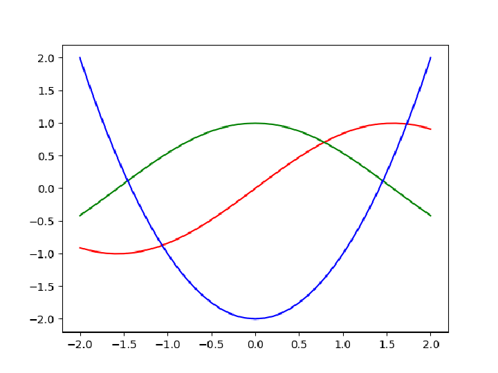
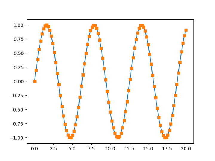
Plot several functions in different colors on the same plot:
Clear the figure:
Alternatively, create several plots with a single command:
Scope (22)
Basic Usage (7)
Plot using the default image format ("PNG"):
Plot a "JPG" image:
Create a basic plot:
Export the plot by specifying the image format as filename extension:
Print the first line of the exported file:
Export by specifying the format as a second argument:
Check the file and delete it:
List file formats available for export:
Export the plot in temporary files in a few of the available formats:
Print the first line of the exported files:
Delete the temporary files:
Plot using the default figure:
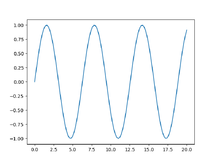
Plot in two figures, starting from a sine in figure 1:
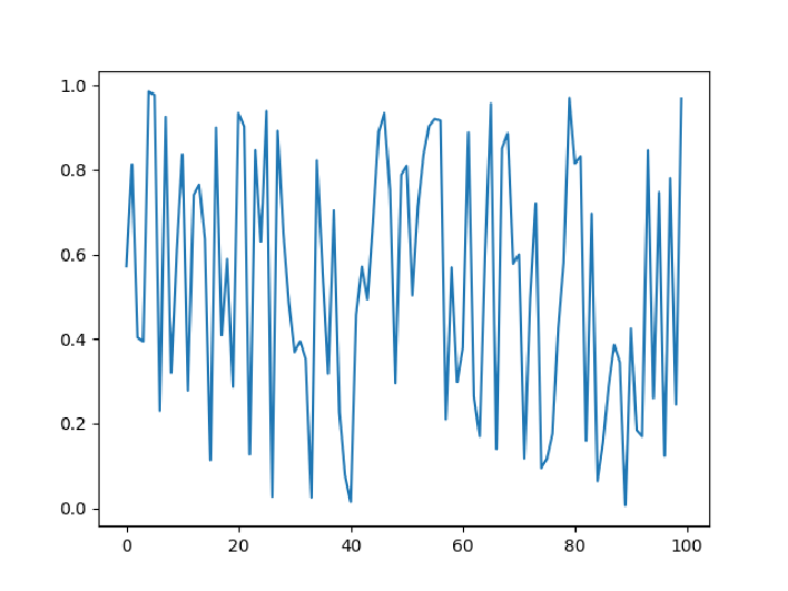
Switch to a new figure 2 and plot some random numbers:
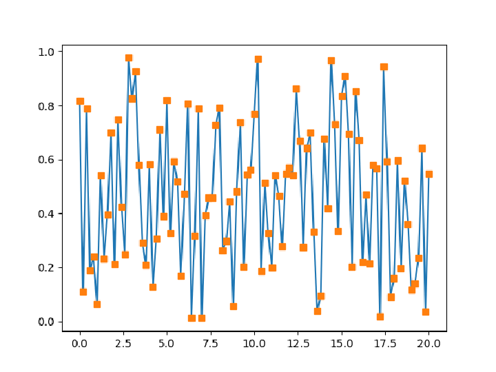
Switch back to figure 1 and plot points:
Make similar changes in figure 2:
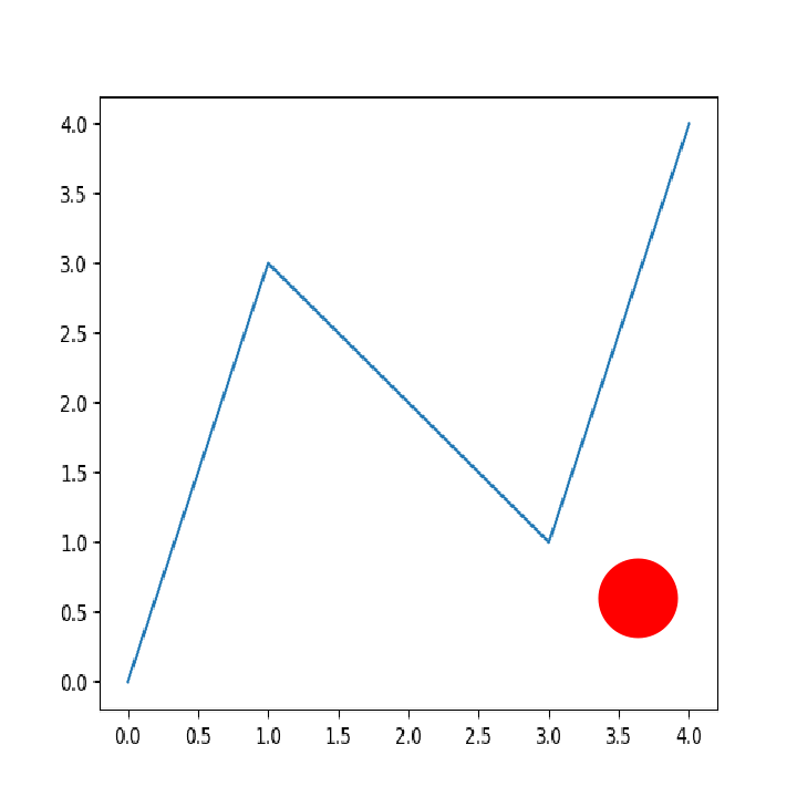
Create a figure with axes with an area where points are specified by coordinates:
Draw some data on the axes:
Show the plot:
Create a new MatplotlibObject:
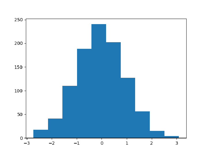
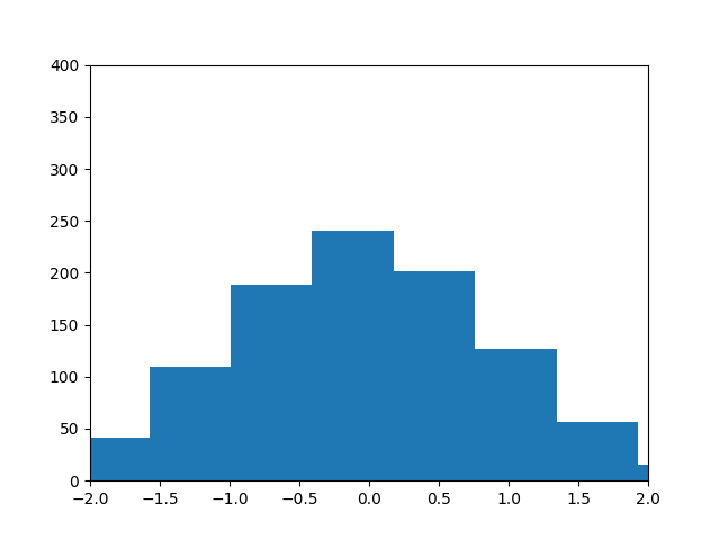
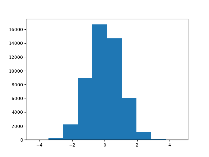
Prepare normally-distributed data and plot a histogram:
Adjust the plot range:
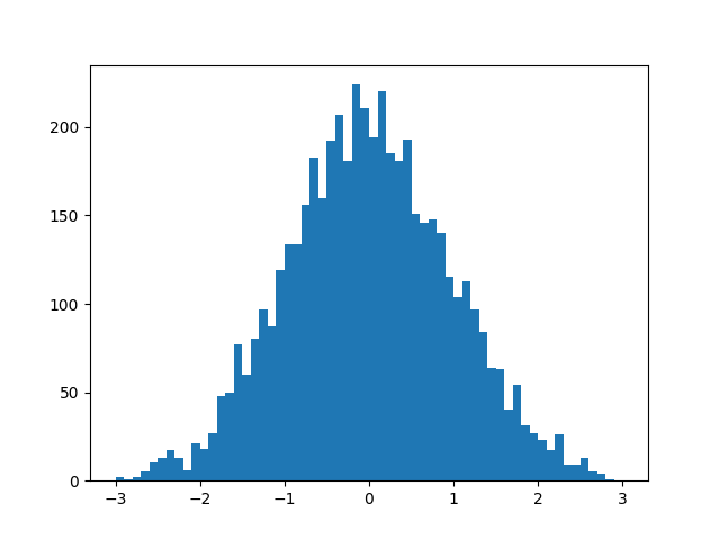
Use the specified Python session:
Create an array of normally distributed values on the Python side:
Create a histogram of the data:
Show the histogram:
Kill the Python session:
Plot Styles (2)
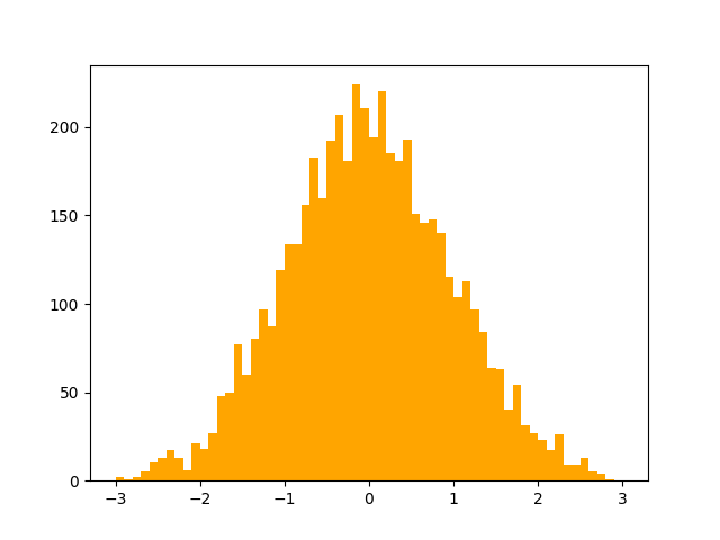
Plot a histogram of some random numbers using the default style:
Clear the figure:
Change the plot style for the histogram (one-off change):
View some of the current style parameters (runtime configuration):
Change one of the style settings in the current Python session to display right-hand side ticks:
Clear the current figure and display the plot with y-labels on both sides:
Restore the defaults:
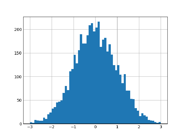
Use a predefined stylesheet:
Show the style settings:
Plot the histogram:
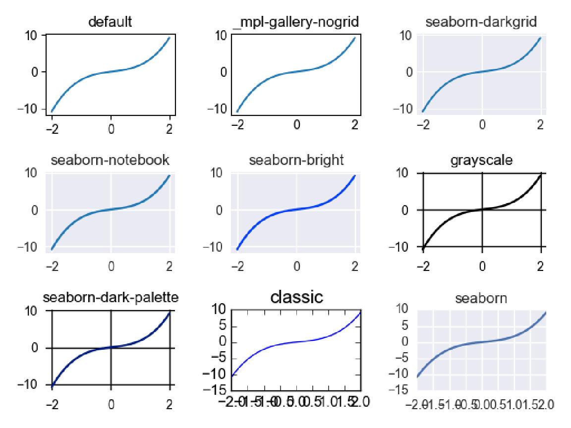
List predefined stylesheets:
Choose a few of the styles:
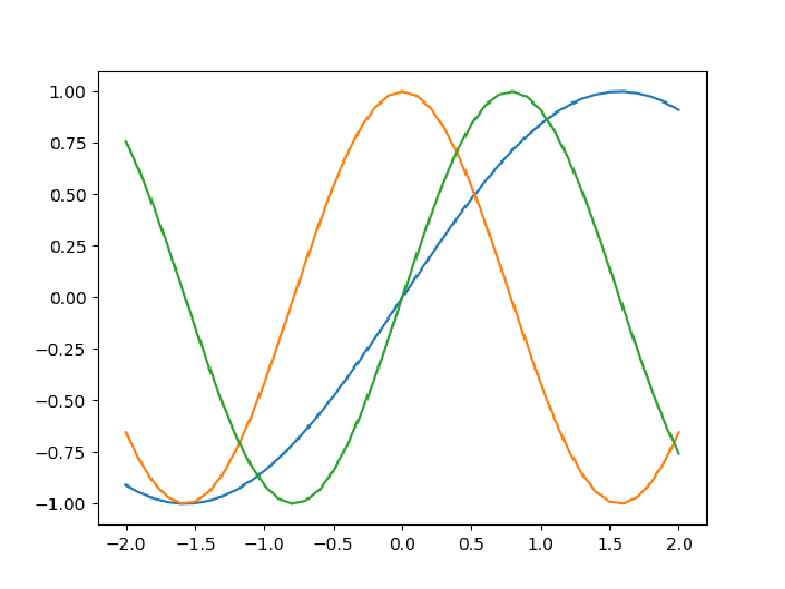
Define a function on a grid:
Plot the function using the stylesheets and display in a 3⨯3 layout:
Basic Plot Types (5)
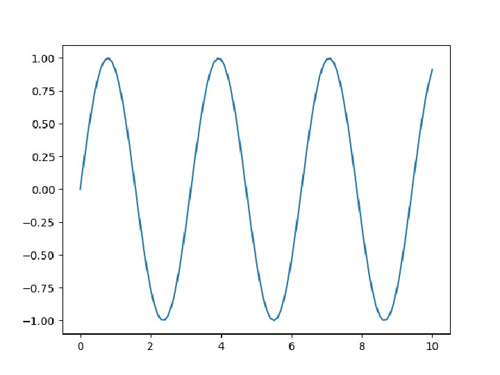
A line plot:
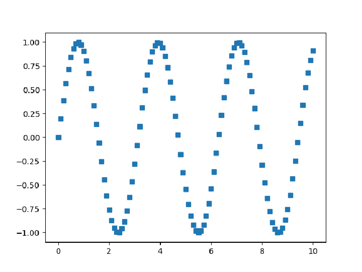
A marker plot:
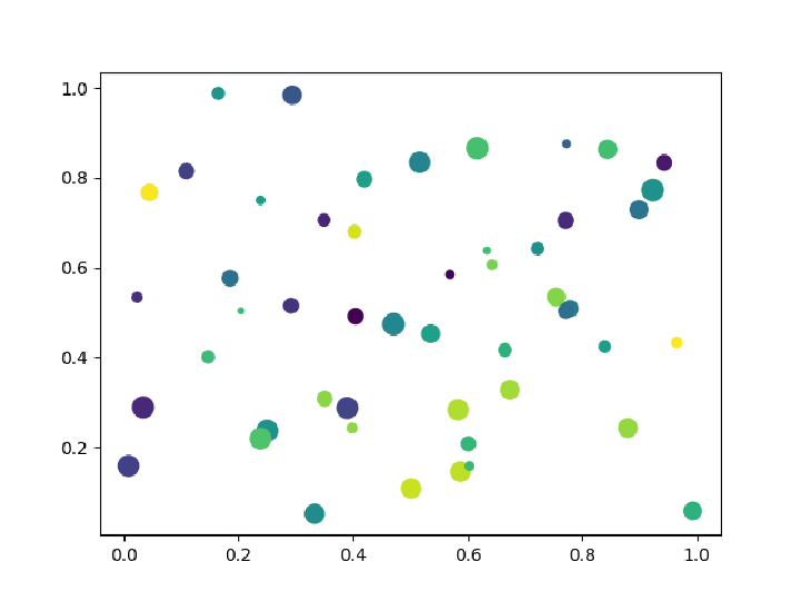
A scatter plot:
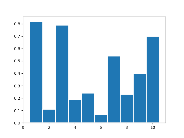
A bar plot:
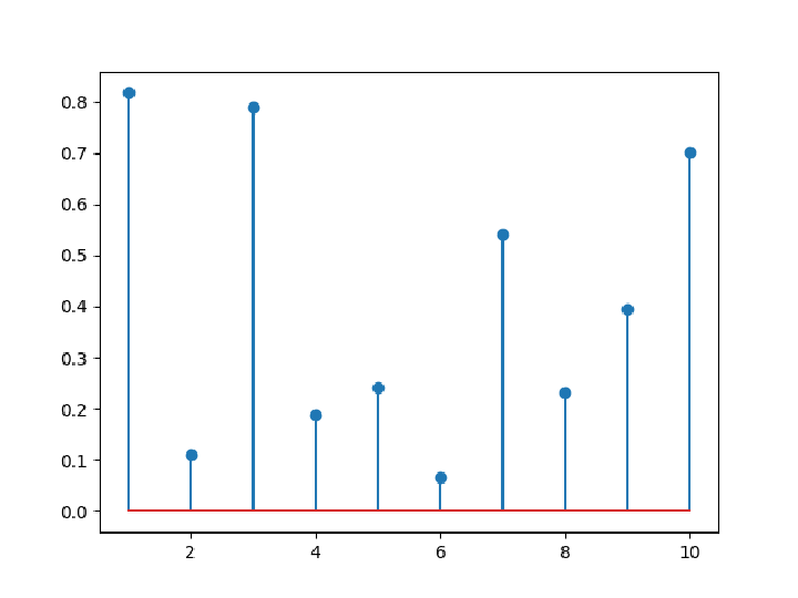
A stem plot of the same data:
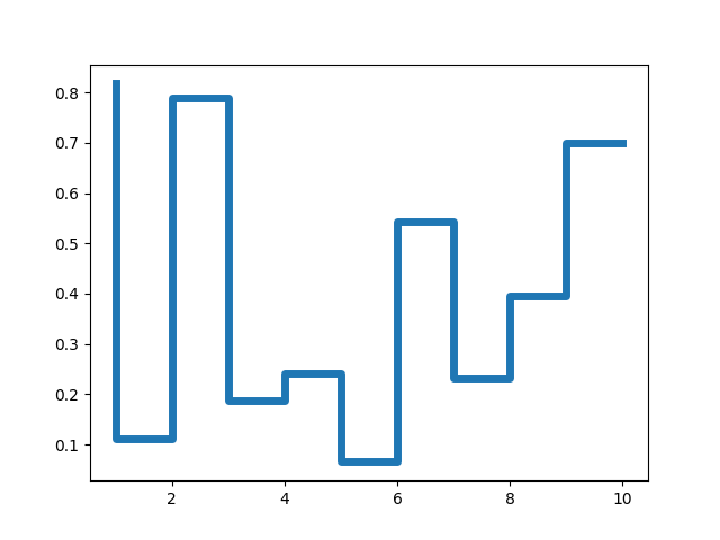
A step plot:
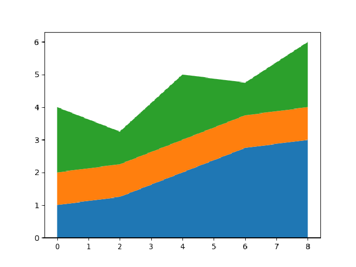
Fill the area between two horizontal curves:
Add a middle line:
Draw a stacked area plot:
Plots of Arrays and Fields (3)
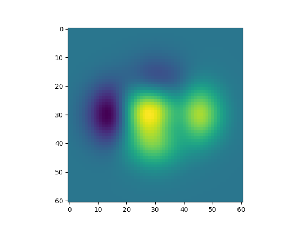
Define a function that returns coordinate matrices constructed from from one-dimensional coordinate vectors of the same length:
Construct coordinate matrices of a raster:
Prepare and show the raster image of the data:
Prepare data for a 2D field of barbs:
Draw a barbs plot:
Adjust the plot range and show the plot:
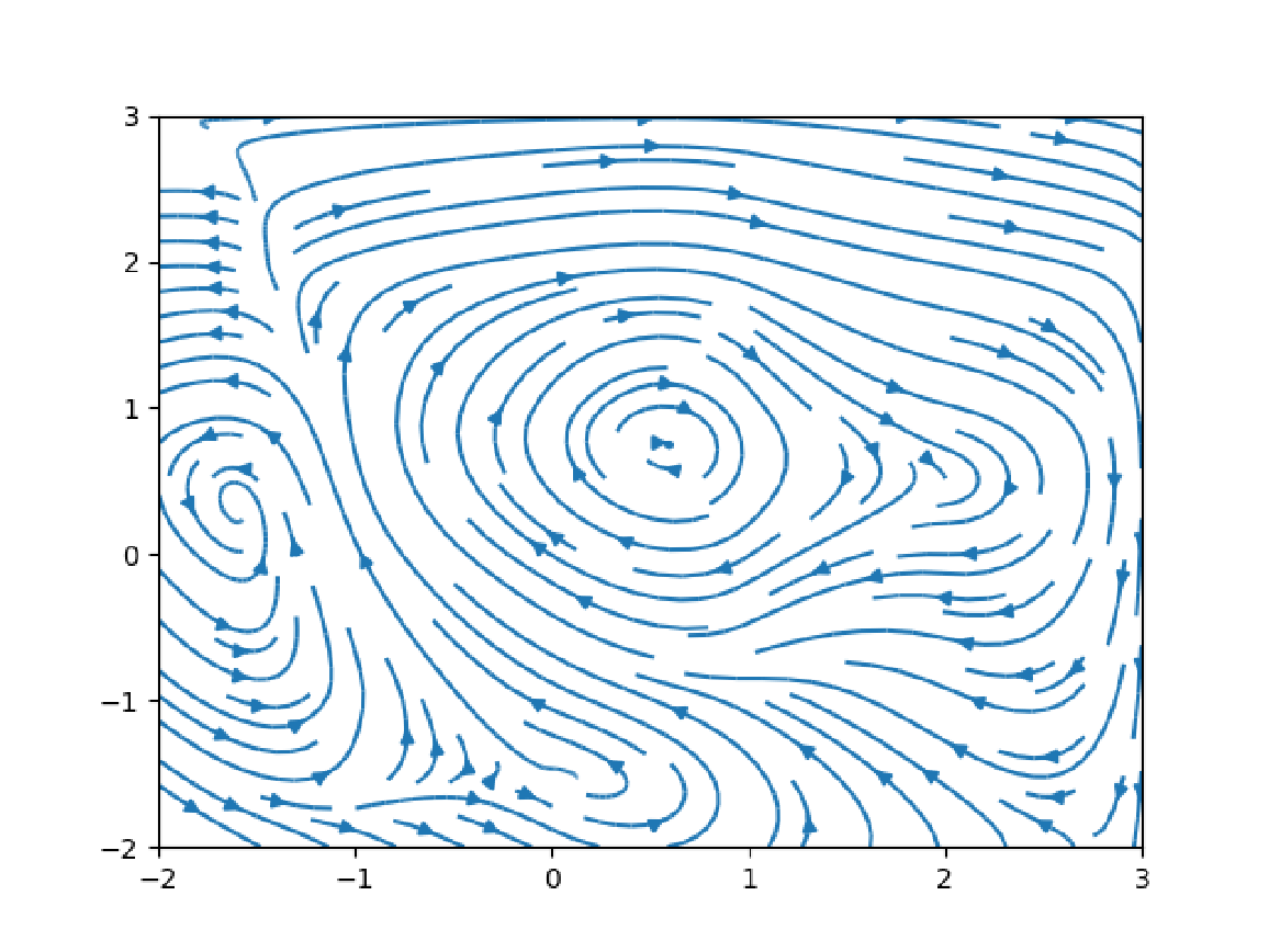
Prepare data for streamlines of a vector flow:
Draw the vector flow:
Statistics Plots (2)
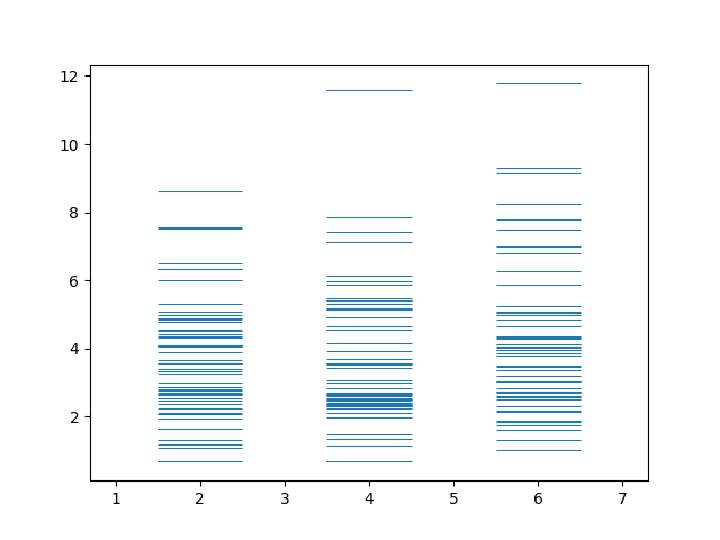
Simulate arrival of customers to a business on different days of the month:
Create and show an event plot:
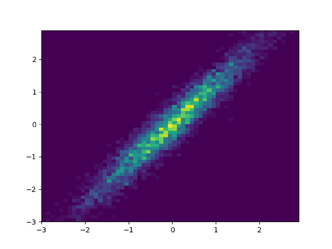
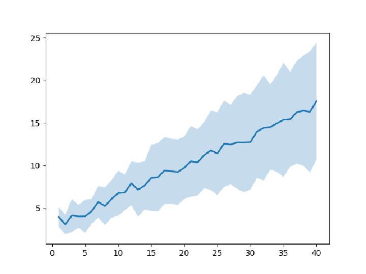
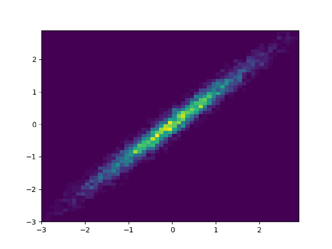
Create a partially correlated data:
Prepare and show a density histogram:
Using Submodules (3)
By default, MatplotlibObject creates a Python object for the submodule pyplot:
Obtain the same result by specifying the submodule explicitly:
Create a PythonObject for the main matplotlib module:
List all available submodules:
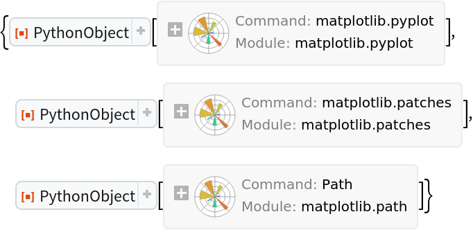
Create Python objects for the main matplotlib module, a few submodules, and the Path class in the submodule path:
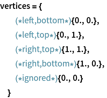
Define a list of vertices:
Use the created path object to define a simple shape using the standard MOVETO, LINETO and CLOSEPOLY commands:
Prepare a figure and axes:
Create a path patch that renders graphics primitives into a canvas and add it to the axes object:
Draw and display the shape:
Applications (6)
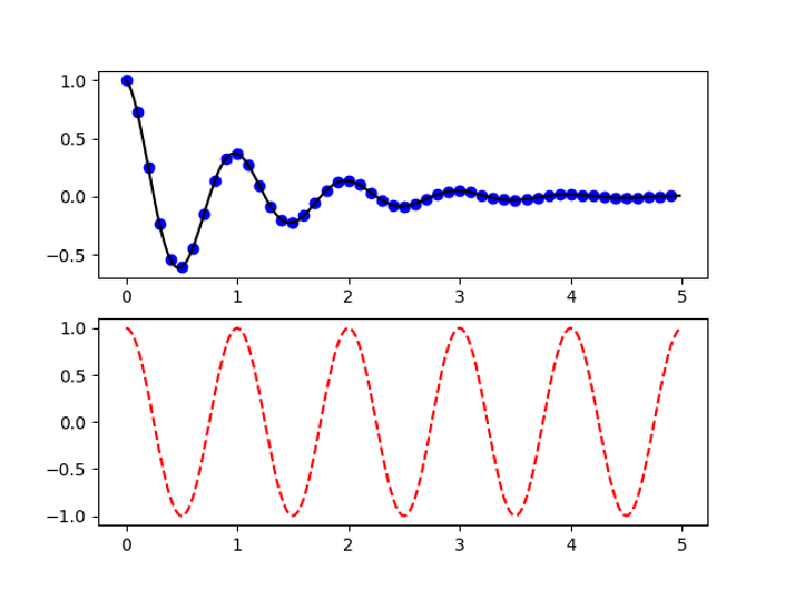
The main use of MatplotlibObject is to plot data in Python without bringing the data to the Wolfram Language. Define a Python function and create NumPy arrays of some data points:
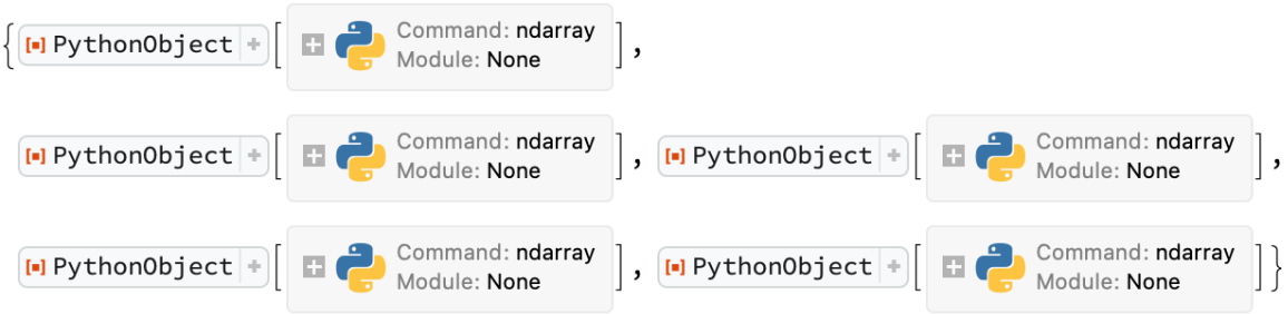
Create references to the NumPy arrays without bringing them to the Wolfram Language:
Create a Figure object and a subplot:
Prepare a plot of points ft1 as blue circles and points ft2 as a black line:
Plot points ct2 as a red dashed line in another subplot:
Display the plots created in Python:
Properties and Relations (4)
MatplotlibObject[…] gives the same result as the resource function PythonObject with a special configuration:
Get information on the main module:
Open the user guide in your default web browser:
The functions available in the pyplot module:
Information on a function:
The web documentation for a function:
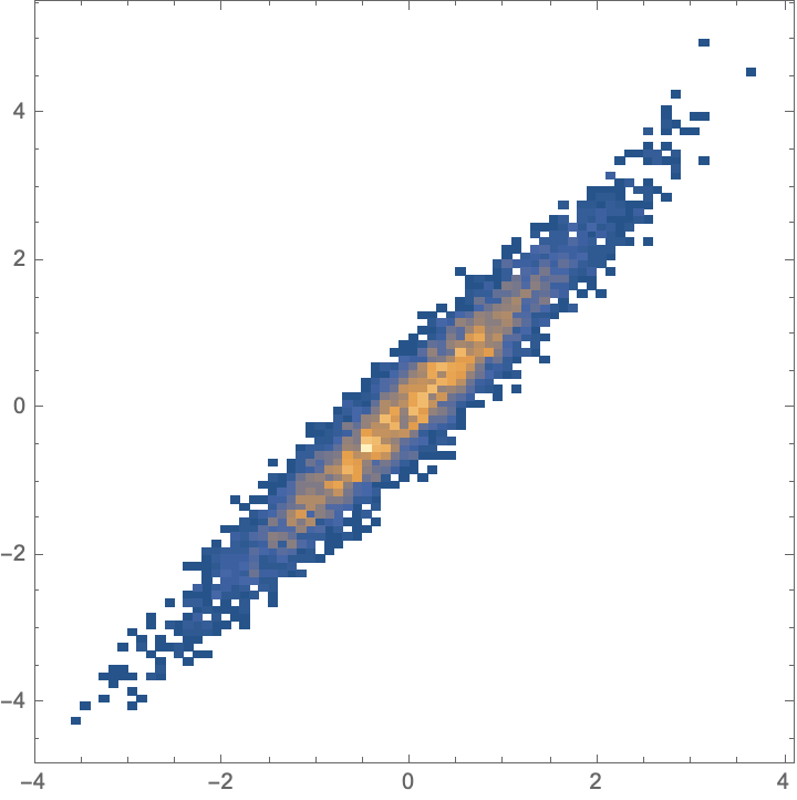
The majority of plots analogous to those in MatplotlibObject are defined directly in the Wolfram Language. Compare, for instance, DensityHistogram and hist2d:
Set up a Python session and a MatplotlibObject:
Create some data in the Python session and plot a 2D histogram in Python:
Show the histogram:
Possible Issues (4)
The effect of options in MatplotlibObject[p,"Show"[…,opts]] is not always the same as in the case of images created in the Wolfram Language:
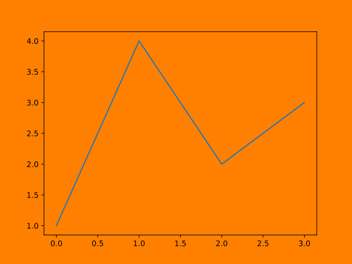
Drawing some data and trying to display the SVG graphics on a colored background does not appear to succeed:
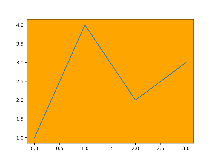
Even though the background can show through if some elements of the graphics are deleted:
Create background in Python instead:


![MapIndexed[Function[{style, part},
plt["style"]["use"[style]]; axes = figure["add_subplot"[rows, cols, part[[1]]], True]; axes["plot"[x, y], True]; axes["set_title"[style], True];
], styles]](https://www.wolframcloud.com/obj/resourcesystem/images/a1b/a1bfb72c-7a7c-4d22-8681-85c885444b46/023881d11761a67c.png)


![ExternalEvaluate[session, "import numpy as np
def f(t):
return np.exp(-t) * np.cos(2*np.pi*t)
t1 = np.arange(0.0, 5.0, 0.1)
t2 = np.arange(0.0, 5.0, 0.02)
ft1 = f(t1)
ft2 = f(t2)
ct2 = np.cos(2*np.pi*t2)
"]](https://www.wolframcloud.com/obj/resourcesystem/images/a1b/a1bfb72c-7a7c-4d22-8681-85c885444b46/56726e2a4695835b.png)