Wolfram Function Repository
Instant-use add-on functions for the Wolfram Language
Function Repository Resource:
Sample from a probability density function using the Markov chain Monte Carlo (MCMC) method
ResourceFunction["MonteCarloSample"][f,p,n] generates n samples from probability density function f starting from point p. | |
ResourceFunction["MonteCarloSample"][f,{p1,…,pm},n] generates samples starting from an ensemble consisting of m points. | |
ResourceFunction["MonteCarloSample"][f,{dist,m},n] uses probability distribution dist as the prior and samples m points from dist as the initial points. | |
ResourceFunction["MonteCarloSample"][f,p,{n,burn}] generates samples but discards the first burn samples. | |
ResourceFunction["MonteCarloSample"][f,p,{n,burn,i}] generates samples and takes every ith sample. |
| Method | Automatic | the MCMC algorithm to use |
| "LogProbability" | False | whether the probability function f is specified on a log scale |
| "TargetAcceptanceRate" | 0.25 | the target rate at which proposed points are accepted for certain methods |
| “ListableFunction" | False | whether the probability function f is listable |
| Parallelization | False | whether parallelization is used in sampling |
| "RandomWalk" | uses a fixed probability distribution for drawing proposals |
| "AdaptiveMetropolis" | use the method of Haario et al. |
| "EMCEE" | use the method of Foreman-Mackey et al. |
| "DifferentialEvolution" | use the method of ter Braak |
| "JumpDistribution" | the symmetrical probability distribution for drawing proposals |
| "InitialScaleMultiplier" | 1 | the initial scale of the step relative to the default one |
| "RandomWalkScale" | 0.1 | the absolute scale of steps when random walk is adopted |
| "StretchScale" | 2 | the maximum scale of the stretch moves |
| "InitialScaleMultiplier" | 2 | the initial scale of the step relative to the default one |
| "RandomnessScale" | 0.001 | the relative scale of randomness of the steps |
Generate 10 samples from a Student t distribution with 3 degrees of freedom:
| In[1]:= |
| Out[1]= |
Generate 1000 samples, discard the first 200 samples, and take every fifth sample:
| In[2]:= |
| Out[2]= |
| In[3]:= |
| Out[3]= | 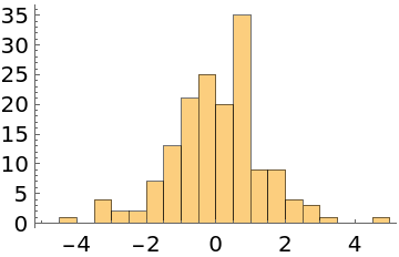 |
Do automatic burn-in removal and thinning instead:
| In[4]:= |
| Out[4]= |
| In[5]:= |
| Out[5]= | 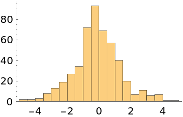 |
Sample from a 2D normal distribution starting from an ensemble consisting of 10 random points:
| In[6]:= |
| Out[6]= |
| In[7]:= |
| Out[7]= | 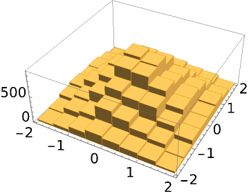 |
Specify a prior in addition to the likelihood function:
| In[8]:= |
| Out[8]= |
| Out[9]= |
| In[10]:= |
| Out[10]= |
| In[11]:= |
| Out[11]= | 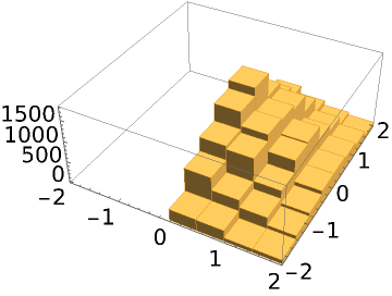 |
The random walk method takes jumps following a normal distribution by default. A custom distribution can also be specified:
| In[12]:= | ![ResourceFunction["MonteCarloSample"][Exp[-#^2/2] &, {0.}, 10, Method -> {"RandomWalk", "JumpDistribution" -> UniformDistribution[{{-0.5, 0.5}}]}]](https://www.wolframcloud.com/obj/resourcesystem/images/ab0/ab096f62-5861-48b2-8f79-9895a37f1701/2c74c576dc36b44b.png) |
| Out[12]= |
The adaptive Metropolis method takes jumps following an adaptive multinormal distribution that is derived from existing samples:
| In[13]:= | ![Short[data = ResourceFunction["MonteCarloSample"][Exp[-#^2/2] &, RandomReal[{-0.05, 0.05}, {10, 1}], 200, Method -> "AdaptiveMetropolis"]]](https://www.wolframcloud.com/obj/resourcesystem/images/ab0/ab096f62-5861-48b2-8f79-9895a37f1701/771955e2aaa4f9d9.png) |
| Out[13]= |
| In[14]:= |
| Out[14]= | 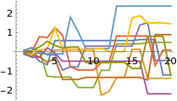 |
The EMCEE and differential evolution methods take jumps being the displacement between two points multiplied by a scale factor. Increasing the number of initial points may improve the performance of these two methods:
| In[15]:= | ![Short[data = ResourceFunction["MonteCarloSample"][Exp[-#^2/2] &, RandomReal[{-1, 1}, {100, 1}], 4000, Method -> "EMCEE"]]](https://www.wolframcloud.com/obj/resourcesystem/images/ab0/ab096f62-5861-48b2-8f79-9895a37f1701/0e427560f2e582b4.png) |
| Out[15]= |
| In[16]:= |
| Out[16]= | 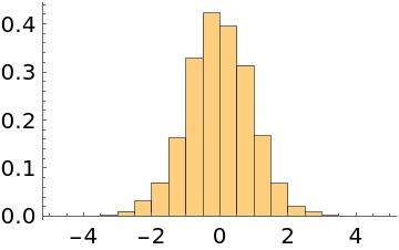 |
When the probability function evaluates to a tiny number, machine numbers may not be able to represent them accurately and the samples do not converge:
| In[17]:= |
| Out[17]= |
| In[18]:= |
| Out[18]= | 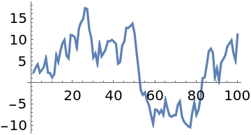 |
"LogProbability"→True indicates that the probability function is on a log scale, and the samples converge to x≈50:
| In[19]:= |
| Out[19]= |
| In[20]:= |
| Out[20]= | 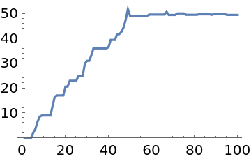 |
Setting the target acceptance rate is only effective for adaptive Metropolis or differential evolution methods. A higher acceptance rate decreases the step size and vice versa:
| In[21]:= | ![Short[data1 = ResourceFunction["MonteCarloSample"][-#^2/2 &, RandomReal[{-1, 1}, {10, 1}], 400, Method -> "AdaptiveMetropolis", "LogProbability" -> True, "TargetAcceptanceRate" -> 0.1]]](https://www.wolframcloud.com/obj/resourcesystem/images/ab0/ab096f62-5861-48b2-8f79-9895a37f1701/64b3563789da2a6a.png) |
| Out[21]= |
| In[22]:= | ![Short[data2 = ResourceFunction["MonteCarloSample"][-#^2/2 &, RandomReal[{-1, 1}, {10, 1}], 400, Method -> "AdaptiveMetropolis", "LogProbability" -> True, "TargetAcceptanceRate" -> 0.9]]](https://www.wolframcloud.com/obj/resourcesystem/images/ab0/ab096f62-5861-48b2-8f79-9895a37f1701/0ef51afaec17dbea.png) |
| Out[22]= |
| In[23]:= |
| Out[23]= | 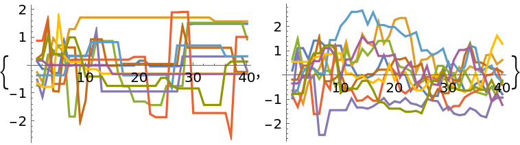 |
If the probability function is listable, specifying "ListableFunction"→True and employing a large number of initial points may significantly improve the performance:
| In[24]:= |
| Out[24]= |
| In[25]:= | ![AbsoluteTiming[
ResourceFunction["MonteCarloSample"][Exp[-#^2/2] &, RandomReal[{-1, 1}, {100, 1}], 10000, "ListableFunction" -> True];]](https://www.wolframcloud.com/obj/resourcesystem/images/ab0/ab096f62-5861-48b2-8f79-9895a37f1701/2535d51ff3401bbe.png) |
| Out[25]= |
Enabling parallelization is only beneficial when the probability function can be run in parallel and each evaluation takes a long time:
| In[26]:= |
| Out[27]= |
| In[28]:= | ![AbsoluteTiming[
ResourceFunction["MonteCarloSample"][prob, RandomReal[{3, 4}, {10, 1}], 40, Parallelization -> True];]](https://www.wolframcloud.com/obj/resourcesystem/images/ab0/ab096f62-5861-48b2-8f79-9895a37f1701/11f0c8e424fce476.png) |
| Out[28]= |
Get the posterior distribution of two parameters in a Student t distribution:
| In[29]:= |
| Out[29]= |
Choose a uniform prior over μ∈[-2,2], σ∈[0,3]:
| In[30]:= |
| Out[31]= |
Run MCMC:
| In[32]:= | ![Short[data = ResourceFunction["MonteCarloSample"][
loglikelihood, {prior, 20}, {10000, Automatic, Automatic}, "LogProbability" -> True]]](https://www.wolframcloud.com/obj/resourcesystem/images/ab0/ab096f62-5861-48b2-8f79-9895a37f1701/1e911bd876bc1e4a.png) |
| Out[32]= |
| In[33]:= |
| Out[33]= | 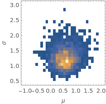 |
The location of the peak in the posterior distribution matches the result given by EstimatedDistribution:
| In[34]:= |
| Out[34]= |
Get the posterior distribution of amplitude, frequency, phase, and mean of a sinusoidal function:
| In[35]:= | ![f[x_] := 1.5 Sin[3.0 x + 1.0] - 0.6
noise := RandomVariate[NormalDistribution[0, 0.25]]
Short[points = Table[{x, Around[f[x] + noise, 0.25]}, {x, RandomReal[{0, 5}, 40]}]]](https://www.wolframcloud.com/obj/resourcesystem/images/ab0/ab096f62-5861-48b2-8f79-9895a37f1701/7bcc99ebfee895fa.png) |
| Out[37]= |
| In[38]:= |
| Out[38]= | 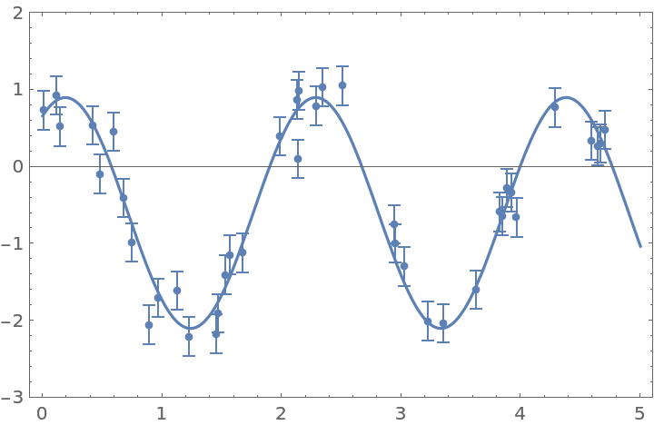 |
The likelihood is derived based on the assumption that each point has a normally distributed error. Define the likelihood, and select the initial points for MCMC around the peak of the likelihood function:
| In[39]:= | ![loglikelihood[a_, \[Omega]_, \[Phi]_, b_] := Evaluate@
Total[-(((a Sin[\[Omega] #1 + \[Phi]] - b) - #2[[1]])^2/(
2 #2[[2]]^2)) & @@@ points]
Short[initial = # + {1.5, 3.0, 1.0, -0.6} & /@ RandomReal[{-0.1, 0.1}, {50, 4}]]](https://www.wolframcloud.com/obj/resourcesystem/images/ab0/ab096f62-5861-48b2-8f79-9895a37f1701/3553d1460090bf37.png) |
| Out[40]= |
Run MCMC:
| In[41]:= | ![Short[data = ResourceFunction["MonteCarloSample"][loglikelihood, initial, {50000, Automatic, Automatic}, Method -> "AdaptiveMetropolis", "LogProbability" -> True, "ListableFunction" -> True]]](https://www.wolframcloud.com/obj/resourcesystem/images/ab0/ab096f62-5861-48b2-8f79-9895a37f1701/5055f2e17e485d85.png) |
| Out[41]= |
The marginal distribution of all four parameters compared to their input values:
| In[42]:= | ![MapThread[
Histogram[#, 20, "PDF", Frame -> True, FrameLabel -> {#2, "PDF"}, Epilog -> {Red, InfiniteLine[{#3, 0}, {0, 1}]}] &, {Transpose@
data, {"amplitude", "frequency", "phase", "mean"}, {1.5, 3.0, 1.0, 0.6}}]](https://www.wolframcloud.com/obj/resourcesystem/images/ab0/ab096f62-5861-48b2-8f79-9895a37f1701/0c58083478c855db.png) |
| Out[42]= | 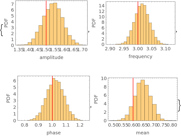 |
The normalization of the probability function does not affect the result:
| In[43]:= | ![normalized[x_] := 1/(\[Pi] (1 + x^2))
unnormalized[x_] := 1/(1 + x^2)
Histogram[Flatten[#], {-3, 3, 0.5}] & /@
{ResourceFunction["MonteCarloSample"][normalized, RandomReal[{-1, 1}, {10, 1}], 8000],
ResourceFunction["MonteCarloSample"][unnormalized, RandomReal[{-1, 1}, {10, 1}], 8000]}](https://www.wolframcloud.com/obj/resourcesystem/images/ab0/ab096f62-5861-48b2-8f79-9895a37f1701/4a6e4aa2733cd99d.png) |
| Out[44]= | 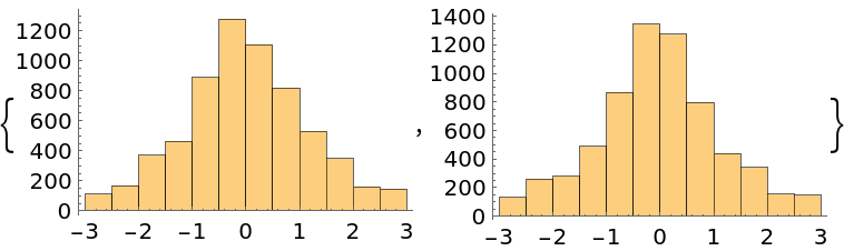 |
If all of the initial points are on an hyperplane, all samples will be on the same hyperplane when the EMCEE or differential evolution method is used:
| In[45]:= |
| Out[45]= |
| In[46]:= | ![Short[data = ResourceFunction["MonteCarloSample"][-(#1^2 + #2^2 + #3^2) &, initial, 500, Method -> "EMCEE", "LogProbability" -> True]]](https://www.wolframcloud.com/obj/resourcesystem/images/ab0/ab096f62-5861-48b2-8f79-9895a37f1701/0b2d8ce437f0aef2.png) |
| Out[46]= |
| In[47]:= |
| Out[47]= | 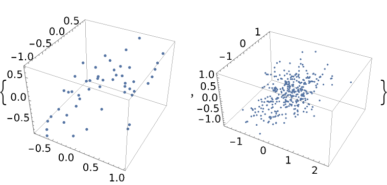 |
Automatic burn-in removal is done by comparing the log-posteriors with the median log-posterior. In some cases, it may keep samples where thermalization has not been reached:
| In[48]:= | ![Short[data1 = Flatten@ResourceFunction["MonteCarloSample"][Exp[-#^2/2] &, RandomReal[{0, 0.0001}, {200, 1}], {20000, Automatic}, Method -> "AdaptiveMetropolis"]]](https://www.wolframcloud.com/obj/resourcesystem/images/ab0/ab096f62-5861-48b2-8f79-9895a37f1701/0ef828078fb39a13.png) |
| Out[48]= |
| In[49]:= |
| Out[49]= |
| In[50]:= |
| Out[50]= | 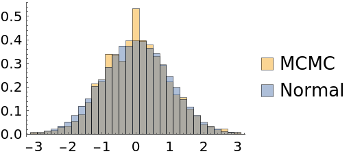 |
To mitigate this problem, place the initial points on a wider range:
| In[51]:= | ![Short[data2 = Flatten@ResourceFunction["MonteCarloSample"][Exp[-#^2/2] &, RandomReal[{-2, 2}, {100, 1}], {20000, Automatic}, Method -> "AdaptiveMetropolis"]]](https://www.wolframcloud.com/obj/resourcesystem/images/ab0/ab096f62-5861-48b2-8f79-9895a37f1701/3f373baee7b82efa.png) |
| Out[51]= |
| In[52]:= |
| Out[52]= | 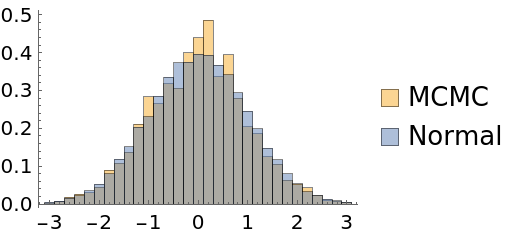 |
This work is licensed under a Creative Commons Attribution 4.0 International License