Function Repository Resource:

LucasCubic

Get the Lucas cubic curve of a triangle

Contributed by: Shenghui Yang (Wolfram Research)

ResourceFunction["LucasCubic"][{p₁,p₂,p₃},{x,y}]

returns the Lucas cubic curve.

Details

Let a, b, c be the side lengths of the reference triangle ABC. Then the equation of the Lucas cubic of triangle ABC in barycentric coordinates (x,y,z) is

where cyc indicates that the sum is taken over all three cyclic permutation of x, y, z.

LucasCubic[Triangle[{p₁,p₂,p₃}],{x,y}] is equivalent to LucasCubic[{p₁,p₂,p₃},{x,y}].

Examples

Basic Examples (2)

Find the Lucas cubic of three triangle vertices:

In[1]:=

$tri = {{13/5, 12/5}, {0, 0}, {3, 0}}; ResourceFunction["LucasCubic"][tri, {\[FormalX], \[FormalY]}]$

Out[2]=

Visualize the cubic curve:

In[3]:=

$ContourPlot[% == 0, {\[FormalX], -1, 6}, {\[FormalY], -3, 4}, ContourLabels -> None]$

Out[3]=

Properties and Relations (1)

The Lucas cubic is closely related to the Thomson cubic:

Possible Issues (1)

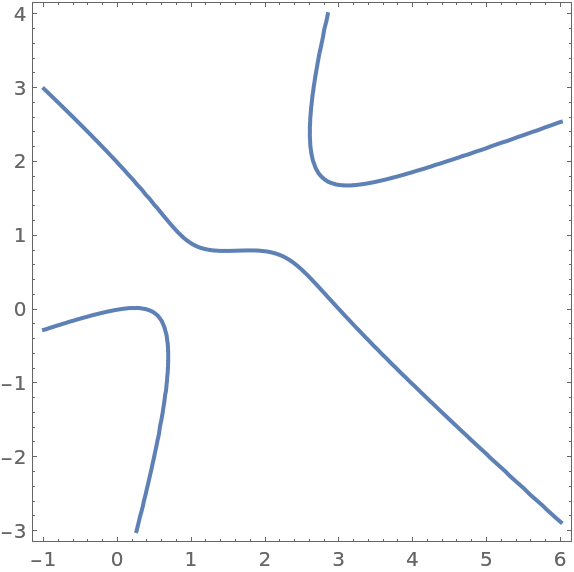Degenerated triangle is not supported:

In[4]:=

$tri = {{0, 0}, {-10, 0}, {2, 0}}; ResourceFunction["LucasCubic"][tri, {\[FormalX], \[FormalY]}]$

Out[5]=

Neat Examples (2)

The circumcenter, orthocenter and Gergonne point and Nagel point of the reference triangle are on the Lucas cubic. The vertices of the reference triangle and that of its anticomplementary triangle are also on the cubic:

In[6]:=

$tri = {{2.6, 2.1}, {0, 0}, {3, 0}}; amt = TriangleConstruct[tri, "AntimedialTriangle"]; amtR = TriangleMeasurement[amt, "Circumradius"]; plotCen = TriangleConstruct[amt, "Circumcenter"][[1]]; ref = { Sequence[{Transparent, EdgeForm[{ Thickness[0.005], Blue}], Triangle[tri]}, {Transparent, EdgeForm[{ Thickness[0.005], Red, Dashed}], amt}, { PointSize[0.017], Blue, TriangleConstruct[tri, "Centroid"]}, { PointSize[0.017], Orange, TriangleConstruct[tri, "Orthocenter"]}, { PointSize[0.017], Red, ResourceFunction["GergonnePoint"][tri]}, { PointSize[0.017], Black, ResourceFunction["NagelPoint"][tri]}]}; xbounds = {plotCen[[1]] - amtR*1.1, plotCen[[1]] + amtR*1.1}; ybounds = {plotCen[[2]] - amtR*1.1, plotCen[[2]] + amtR*1.1}; Legended[ ContourPlot[ Evaluate[ ResourceFunction["LucasCubic"][tri, {\[FormalX], \[FormalY]}] == 0], {\[FormalX], Sequence @@ xbounds}, {\[FormalY], Sequence @@ ybounds}, Sequence[ Epilog -> ref, AspectRatio -> Dot[ybounds, {-1, 1}]/Dot[xbounds, {-1, 1}], ContourLabels -> None, PlotPoints -> 20]], PointLegend[ Sequence[{Blue, Orange, Red, Black}, {"Circumcenter", "Orthocenter", "Gergonne", "Nagel"}]]]$

Out[7]=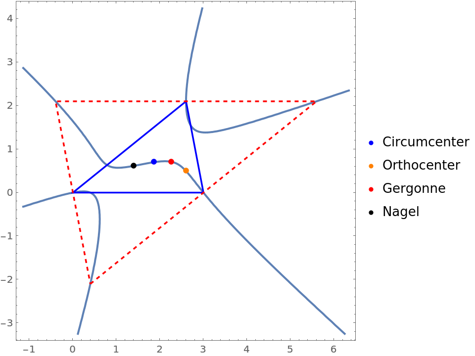

Direct computation of three asymptotes:

In[8]:=

$tri = {{13/5, 12/5}, {0, 0}, {3, 0}}; ResourceFunction["LucasCubic"][tri, {\[FormalX], \[FormalY]}]$

Out[9]=

Solve for y in terms of x:

In[10]:=

$sol = Solve[% == 0, \[FormalY]];$

Extract the constant term and the linear term for each result:

In[11]:=

$asym = (Chop@*N@ Asymptotic[Evaluate[\[FormalY] /. #], {\[FormalX], Infinity, 2}, Assumptions -> \[FormalX] > 0]) /. Times[ele_, Power[\[FormalX], n_ /; (n < 0)]] :> 0 & /@ sol$

Out[11]=

Visualize the curve and its asymptotes:

In[12]:=

$Module[{amt, amtR, plotCen, ref, xbounds, ybounds}, (amt = TriangleConstruct[ tri, "AntimedialTriangle"]; amtR = TriangleMeasurement[ amt, "Circumradius"]; plotCen = Part[ TriangleConstruct[amt, "Circumcenter"], 1]; ref = {{Transparent, EdgeForm[{ Thickness[0.005], Blue}], Triangle[tri]}, {Transparent, EdgeForm[{ Thickness[0.005], Red, Dashed}], amt}}; xbounds = {Part[ plotCen, 1] - amtR 1.3, Part[plotCen, 1] + amtR 1.1}; ybounds = {Part[ plotCen, 2] - amtR 1.1, Part[plotCen, 2] + amtR 1.3}); ContourPlot[Evaluate[ {ResourceFunction["LucasCubic"][tri, {\[FormalX], \[FormalY]}] == 0, Splice[\[FormalY] == # & /@ asym]} ], Sequence[{\[FormalX], Apply[Sequence, xbounds]}, {\[FormalY], Apply[Sequence, ybounds]}, Epilog -> ref, AspectRatio -> Dot[ybounds, {-1, 1}]/Dot[xbounds, {-1, 1}], ContourLabels -> None, PlotPoints -> 20]]]$

Out[12]=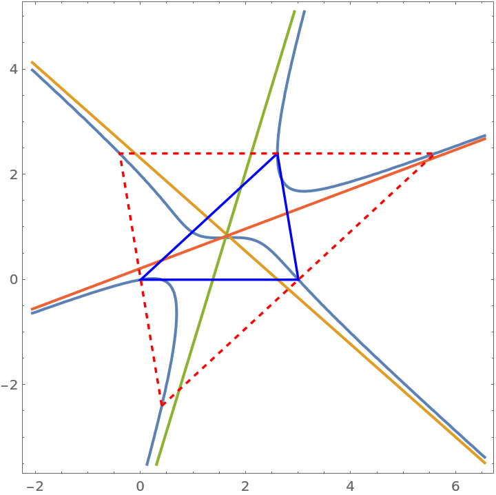

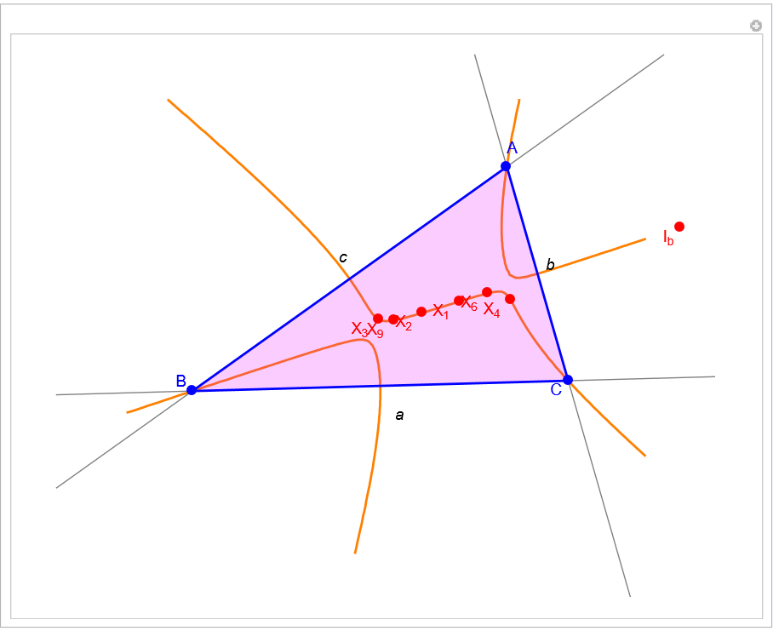
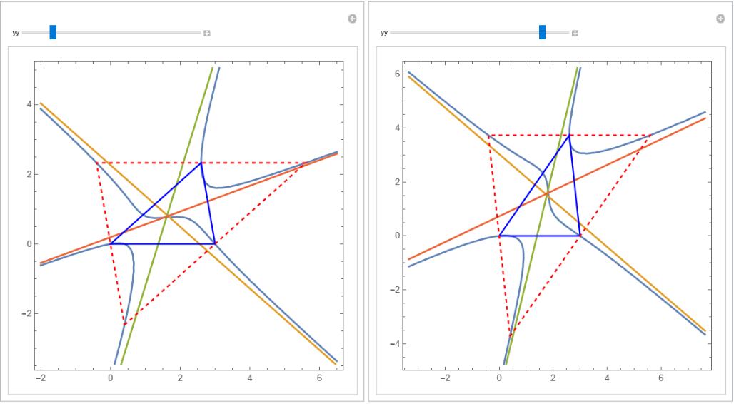
Or we can wrap everything into a Manipulate function:

In[13]:=

$Manipulate[DynamicModule[{amt, amtR, plotCen, ref, xbounds, ybounds, tri, sol, asym}, tri = {{13/5, yy}, {0, 0}, {3, 0}}; sol = Quiet[ Solve[LucasCubic[ tri, {\[FormalX], \[FormalY]}] == 0, \[FormalY]]]; asym = Map[ ReplaceAll[ Composition[Chop, N][ Asymptotic[ Evaluate[ ReplaceAll[\[FormalY], #]], {\[FormalX], Infinity, 2}, Assumptions -> \[FormalX] > 0]], Pattern[ele, Blank[]] \[FormalX]^Condition[ Pattern[n, Blank[]], n < 0] :> 0]& , sol]; amt = TriangleConstruct[ tri, "AntimedialTriangle"]; amtR = TriangleMeasurement[ amt, "Circumradius"]; plotCen = Part[ TriangleConstruct[amt, "Circumcenter"], 1]; ref = {{Transparent, EdgeForm[{ Thickness[0.005], Blue}], Triangle[tri]}, {Transparent, EdgeForm[{ Thickness[0.005], Red, Dashed}], amt}}; xbounds = {Part[ plotCen, 1] - amtR 1.3, Part[plotCen, 1] + amtR 1.1}; ybounds = {Part[ plotCen, 2] - amtR 1.1, Part[plotCen, 2] + amtR 1.3}; With[{expr = {LucasCubic[ tri, {\[FormalX], \[FormalY]}] == 0, Splice[ Map[\[FormalY] == #& , asym]]}}, ContourPlot[expr, {\[FormalX], Apply[Sequence, xbounds]}, {\[FormalY], Apply[Sequence, ybounds]}, Epilog -> ref, AspectRatio -> Dot[ybounds, {-1, 1}]/Dot[xbounds, {-1, 1}], ContourLabels -> None, PlotPoints -> 10]]], {yy, 2, 4}, Sequence[ TrackedSymbols :> {yy}, SynchronousUpdating -> False, SaveDefinitions -> True]]$

Publisher

Shenghui Yang

Version History

1.0.0 – 16 June 2023

Source Metadata

Citation:
- van Lamoen, Floor. "Lucas Cubic." From MathWorld--A Wolfram Web Resource, created by Eric W. Weisstein.

Related Resources

License Information

This work is licensed under a Creative Commons Attribution 4.0 International License

Wolfram Function Repository

LucasCubic

Details