Wolfram Function Repository
Instant-use add-on functions for the Wolfram Language
Function Repository Resource:
Provide an indexed priority queue data structure with its standard operations
ResourceFunction["IndexedQueue"][] returns an indexed priority queue initialized with default settings. | |
ResourceFunction["IndexedQueue"][{"InitialSize"→size,"NullElement"→null,"ComparisonFunction"→comp},"Initialize"] returns an indexed queue initialized to have length size, null element null and comparison function comp. | |
ResourceFunction["IndexedQueue"][inits,vals,"Initialize"] returns an indexed queue initialized with parameters in inits and containing values vals. | |
ResourceFunction["IndexedQueue"][queue,"Dequeue"] returns a list containing the index and value of the topmost element in queue. | |
ResourceFunction["IndexedQueue"][queue,value,"Enqueue"] places value in queue, associating to it an index equal to the current queue length plus one. | |
ResourceFunction["IndexedQueue"][queue,index,"Remove"] removes the element indexed by index from queue. | |
ResourceFunction["IndexedQueue"][queue,index,value,"UpdateValue"] replaces the current value of element index with value, reordering queue as needed. | |
ResourceFunction["IndexedQueue"][queue,"Length"] gives the number of elements in queue. | |
ResourceFunction["IndexedQueue"][queue,"Peek"] gives the value of the topmost element in queue. | |
ResourceFunction["IndexedQueue"][queue,"TopIndex"] gives the index of the topmost element in queue. | |
ResourceFunction["IndexedQueue"][queue,keyindex,"Value"] gives the value associated to the element indexed by keyindex, or the null value if it is not present. |
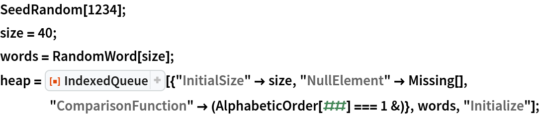
Initialize a priority queue (aka ordered heap) with 20 random reals between -1 and 1:

Check the size:
| In[1]:= |
| Out[1]= |
Check the value of the largest element:
| In[2]:= |
| Out[2]= |
Add 80 more random values to the heap:
Recheck length and largest value:
| In[3]:= |
| Out[3]= |
When we dequeue elements one-by-one, the result is a sorted list of values; this method is called the "heap-sort" algorithm:
| In[4]:= | ![sorted = Reap[
While [! ResourceFunction["IndexedQueue"][heap, "EmptyQ"], Sow[ResourceFunction["IndexedQueue"][heap, "Dequeue"]]]][[2, 1]];
sorted[[All, 2]]](https://www.wolframcloud.com/obj/resourcesystem/images/493/493fb51a-b052-49fe-8c8e-c8bcbc79de88/34a0ccc49f5d464b.png) |
| Out[4]= |  |
Check that it is indeed empty:
| In[5]:= |
| Out[5]= |
An alternative check is that the length is zero:
| In[6]:= |
| Out[6]= |
Check that the result is correctly sorted largest-to-smallest:
| In[7]:= |
| Out[7]= |
IndexedQueue can work with any data type for which an ordering exists, such as words with alphabetical order:
Now sort them in dictionary order by dequeuing, returning both original positions and values:
| In[8]:= | ![sortedwords = Reap[While [! ResourceFunction["IndexedQueue"][heap, "EmptyQ"], Sow[ResourceFunction["IndexedQueue"][heap, "Dequeue"]]]][[2, 1]]](https://www.wolframcloud.com/obj/resourcesystem/images/493/493fb51a-b052-49fe-8c8e-c8bcbc79de88/20efed8a3e778493.png) |
| Out[8]= |  |
For a queue of size n, we expect speed proportional to n log n for creating and removing all elements. We test this by timing a basic sorting, then doubling size twice.
Use a queue to enqueue 10000 random values:
| In[9]:= | ![defaultNames = {"InitialSize", "NullElement", "ComparisonFunction"};
size = 10^4;
vals = RandomReal[{-1, 1}, size];
Timing[heap = ResourceFunction["IndexedQueue"][
Thread[defaultNames -> {size, 0., Greater}], vals, "Initialize"];]](https://www.wolframcloud.com/obj/resourcesystem/images/493/493fb51a-b052-49fe-8c8e-c8bcbc79de88/00a70c9e16286e6d.png) |
| Out[9]= |
Now dequeue all elements:
| In[10]:= | ![Timing[sorted = Reap[While [! ResourceFunction["IndexedQueue"][heap, "EmptyQ"], Sow[ResourceFunction["IndexedQueue"][heap, "Dequeue"]]]][[2, 1]];]](https://www.wolframcloud.com/obj/resourcesystem/images/493/493fb51a-b052-49fe-8c8e-c8bcbc79de88/5a0f9eed248815ce.png) |
| Out[10]= |
| In[11]:= |
| Out[11]= |
Double the size and check enqueing and dequeing timings:
| In[12]:= | ![(* Evaluate this cell to get the example input *) CloudGet["https://www.wolframcloud.com/obj/bf59a93d-868c-468c-a16b-081ec72c4fa2"]](https://www.wolframcloud.com/obj/resourcesystem/images/493/493fb51a-b052-49fe-8c8e-c8bcbc79de88/407288c5f92a9305.png) |
| Out[12]= |
Again double the size and check enqueing and dequeing timings:
| In[13]:= | ![(* Evaluate this cell to get the example input *) CloudGet["https://www.wolframcloud.com/obj/35105f07-1ea6-4c80-87f4-ee09c9d5df6b"]](https://www.wolframcloud.com/obj/resourcesystem/images/493/493fb51a-b052-49fe-8c8e-c8bcbc79de88/38c8fc9ba15551f1.png) |
| Out[13]= |
Attempting to dequeue from an empty queue gives the default element:

| Out[13]= |
IndexedQueue has the same asymptotic complexity as the resource function PriorityQueue, but it has a larger constant factor due to the extra work in handling enqueuing and dequeuing.
Define a timing test for purposes of comparing IndexedQueue with PriorityQueue:
Create a set of 10000 random real values:

Time enqueuing and dequeuing using IndexedQueue:
| In[14]:= |
| Out[14]= |
Compare to enqueuing and dequeuing using PriorityQueue:
| In[15]:= |
| Out[15]= |
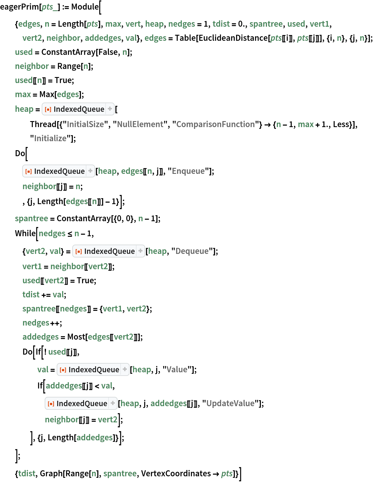
A minimum spanning tree for a connected graph is a tree that connects every vertex, has no cycles and is of minimal total edge weight. The "eager" version of Prim's method for computing the minimum spanning tree of a connected, weighted undirected graph works as follows. Start with any vertex. For any edge from that vertex, enqueue the vertex it connects to with value set to the edge weight. Iteratively remove from the queue the vertex of lowest edge weight and add it to the spanning tree under construction. Then iterate over the vertices connected to that vertex. Ignore those that already are in the tree. Enqueue with edge weight those that are not already in the queue. For a vertex currently in the queue, update the value if the edge weight is less than that which was previously associated to that vertex. For a graph of V vertices and E edges the complexity is O(E log V).
Code for the eager form of Prim's algorithm, specialized to a complete graph with edge weights as pairwise distances between planar points:
Create an example set of points:
| In[16]:= | ![SeedRandom[1234];
nverts = 250;
ListPlot[pts = RandomReal[{-10, 10}, {nverts, 2}]]](https://www.wolframcloud.com/obj/resourcesystem/images/493/493fb51a-b052-49fe-8c8e-c8bcbc79de88/453c5b9cde8ab2da.png) |
| Out[16]= | 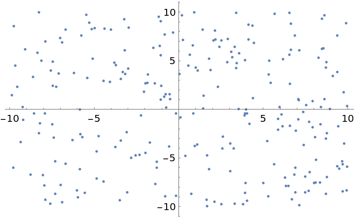 |
Find the minimal spanning tree and total edge weight:
| In[17]:= |
| Out[17]= |
Check the total edge weight:
| In[18]:= |
| Out[18]= |
Plot the spanning tree:
| In[19]:= |
| Out[19]= | 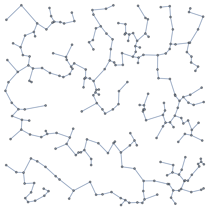 |
Double the vertex count and repeat:
| In[20]:= | ![nverts *= 2;
pts = RandomReal[{-10, 10}, {nverts, 2}];
Timing[{tdist, treegraph} = eagerPrim[pts]]](https://www.wolframcloud.com/obj/resourcesystem/images/493/493fb51a-b052-49fe-8c8e-c8bcbc79de88/1cc097ebe3eeadb3.png) |
| Out[20]= | 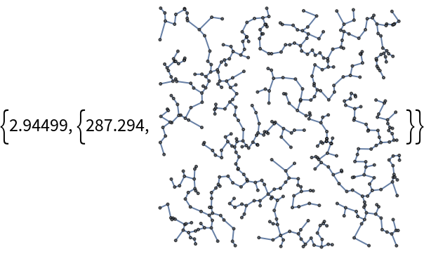 |
Double again:
| In[21]:= | ![nverts *= 2;
pts = RandomReal[{-10, 10}, {nverts, 2}];
Timing[{tdist, treegraph} = eagerPrim[pts]]](https://www.wolframcloud.com/obj/resourcesystem/images/493/493fb51a-b052-49fe-8c8e-c8bcbc79de88/6775c48527286426.png) |
| Out[21]= | 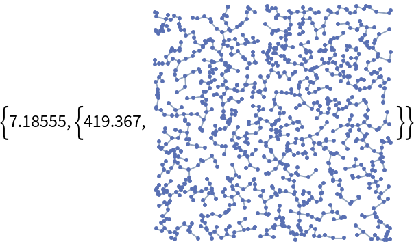 |
Using the built-in Prim method is an order of magnitude faster:
| In[22]:= | ![edges = Flatten[
Table[UndirectedEdge[i, j], {i, nverts - 1}, {j, i + 1, nverts}]];
edgeweights = Flatten[Table[
EuclideanDistance[pts[[i]], pts[[j]]], {i, nverts - 1}, {j, i + 1,
nverts}]];
gr = Graph[Range[nverts], edges, EdgeWeight -> edgeweights, VertexCoordinates -> pts];
Timing[msp = FindSpanningTree[gr, Method -> "Prim"]]](https://www.wolframcloud.com/obj/resourcesystem/images/493/493fb51a-b052-49fe-8c8e-c8bcbc79de88/1e07e3b5fa96d192.png) |
| Out[22]= | 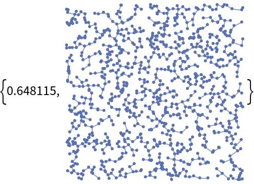 |
A vertex cover for a graph is a subset of vertices that hit all edges. Stated differently, every edge must have at least one endpoint in the cover. A cover with the minimal number of vertices is called a minimal cover. An approximate minimal cover can be found efficiently using a greedy algorithm as follows. First choose a vertex that hits the most edges, and remove those edges from consideration. This means we decrement the edge counts of all vertices connected to the one that was selected. Iteratively remove a vertex hitting the greatest number of remaining edges, and decrement edge counts of vertices connected to the one selected. Continue until no edges remain unhit. This can be implemented efficiently using an indexed priority queue.
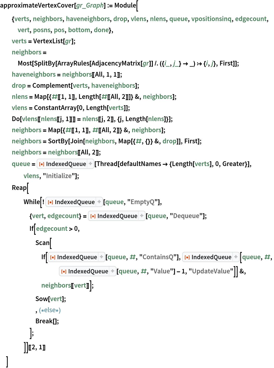
Implement a greedy-with-updates approximate vertex cover using an indexed queue:
Create a random graph with 30 vertices and 80 edges:
| In[23]:= |
| Out[23]= | 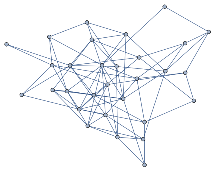 |
Find an approximate vertex cover for this graph:
| In[24]:= |
| Out[24]= |
Check that it is a cover:
| In[25]:= |
| Out[25]= |
Compare the length to the actual minimal cover length:
| In[26]:= |
| Out[26]= |
Time this for a much larger random graph:
| In[27]:= | ![SeedRandom[1234];
gr2 = RandomGraph[{3000, 12000}];
Timing[ac2 = approximateVertexCover[gr2];]](https://www.wolframcloud.com/obj/resourcesystem/images/493/493fb51a-b052-49fe-8c8e-c8bcbc79de88/533adeac5ca48b56.png) |
| Out[27]= |
Check that it is a cover and find the length:
| Out[27]= |
| Out[27]= |
A method used in the resource function ApproximateVertexCover is substantially similar to the one above:
| In[28]:= |
| Out[28]= |
This work is licensed under a Creative Commons Attribution 4.0 International License