Details
Priority queues can be used for sorting by a given ordering function.
Priority queues are also used in the implementation of
Prim's algorithm for computing minimum spanning trees.
The default values for
"InitialSize",
"NullElement" and
"ComparisonFunction" are 16,
Missing["empty slot"] and
Greater, respectively.
"Initialize" can be omitted whenever the first argument is a list of three initialization settings.
In ResourceFunction["PriorityQueue"][queue,value,"Enqueue"], the explicit "Enqueue" can be omitted.
In ResourceFunction["PriorityQueue"][queue,operation], the allowed values of operation are "Length", "EmptyQ", "Dequeue" and "Peek", which perform the following actions:
| "Length" | gives the number of elements currently in the queue |
| "EmptyQ" | gives True if the queue contains no elements, and gives False otherwise |
| "Dequeue" | removes the largest element from the queue and returns its value |
| "Peek" | gives the largest value without removing it from the queue |
In ResourceFunction["PriorityQueue"][queue], the operation "Dequeue" is assumed. In typical usage, one would remove and store the largest element by doing topval=ResourceFunction["PriorityQueue"][queue,"Dequeue"]. Dequeuing all elements from a heap results in a list sorted according to the specified ordering function.
This implementation of priority queues uses binary heaps; this is a common technique.
In binary heap implementations such as this one, each element in a priority queue has either zero, one or two children. If the jthelement has children, they will be located at positions 2j and 2j+1 (with the latter position empty if there is ony one child). Elements are contiguous in the sense that there is never a hole (empty slot) until after the last element.
Each child is ordered less than its parent, but the children do not satisfy a prescribed order with respect to one another.
A priority queue is similar to a binary tree with breadth-first ordering (children considered lower than parents), except children are not always placed in their relative ordering.
Generally, a priority queue is an array of fixed size, so adding and removing elements do not incur memory allocation or deallocation.
The one exception is when adding an element to a queue that is at capacity, at which point the heap size is doubled.
ResourceFunction["PriorityQueue"] has the attribute
HoldFirst.
![SeedRandom[1234];
heap = ResourceFunction[
"PriorityQueue"][{"InitialSize" -> 16, "NullElement" -> Missing[], "ComparisonFunction" -> Greater}, inits = RandomReal[{-1, 1}, 20]];](https://www.wolframcloud.com/obj/resourcesystem/images/3d3/3d37845d-6f9c-442b-8de4-6e83503818e7/3d34fa5fad663fae.png)
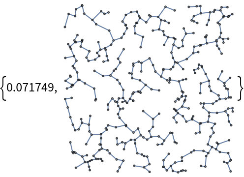
![sorted = Reap[
While [! ResourceFunction["PriorityQueue"][heap, "EmptyQ"], Sow[ResourceFunction["PriorityQueue"][heap, "Dequeue"]]]][[2, 1]]](https://www.wolframcloud.com/obj/resourcesystem/images/3d3/3d37845d-6f9c-442b-8de4-6e83503818e7/505332a24755248e.png)

![SeedRandom[1234];
size = 40;
words = RandomWord[size];
heap = ResourceFunction[
"PriorityQueue"][{"InitialSize" -> size, "NullElement" -> Missing[], "ComparisonFunction" -> (AlphabeticOrder[##] === 1 &)}, words];](https://www.wolframcloud.com/obj/resourcesystem/images/3d3/3d37845d-6f9c-442b-8de4-6e83503818e7/60c68793d446a6cd.png)
![sortedwords = Reap[While [! ResourceFunction["PriorityQueue"][heap, "EmptyQ"], Sow[ResourceFunction["PriorityQueue"][heap, "Dequeue"]]]][[2, 1]]](https://www.wolframcloud.com/obj/resourcesystem/images/3d3/3d37845d-6f9c-442b-8de4-6e83503818e7/5108dc5483af430c.png)

![defaultNames = {"InitialSize", "NullElement", "ComparisonFunction"};
size = 10^4;
vals = RandomReal[{-1, 1}, size];
Timing[heap = ResourceFunction["PriorityQueue"][
Thread[defaultNames -> {size, 0., Greater}], vals, "Initialize"];]](https://www.wolframcloud.com/obj/resourcesystem/images/3d3/3d37845d-6f9c-442b-8de4-6e83503818e7/0d8a41f3f3ad18e7.png)
![Timing[sorted = Reap[While [! ResourceFunction["PriorityQueue"][heap, "EmptyQ"], Sow[ResourceFunction["PriorityQueue"][heap, "Dequeue"]]]][[2, 1]];]](https://www.wolframcloud.com/obj/resourcesystem/images/3d3/3d37845d-6f9c-442b-8de4-6e83503818e7/7cd337bb237f983a.png)
![(* Evaluate this cell to get the example input *) CloudGet["https://www.wolframcloud.com/obj/60c679fa-b76f-4f0c-af03-f8cc5803a130"]](https://www.wolframcloud.com/obj/resourcesystem/images/3d3/3d37845d-6f9c-442b-8de4-6e83503818e7/60e543571ea7c4ed.png)
![(* Evaluate this cell to get the example input *) CloudGet["https://www.wolframcloud.com/obj/a5fadf69-3cbb-4c84-bf5a-3ccf0674d7d3"]](https://www.wolframcloud.com/obj/resourcesystem/images/3d3/3d37845d-6f9c-442b-8de4-6e83503818e7/2be7592a95f351b4.png)
![q = ResourceFunction["PriorityQueue"][];
ResourceFunction["PriorityQueue"][q, "Dequeue"]](https://www.wolframcloud.com/obj/resourcesystem/images/3d3/3d37845d-6f9c-442b-8de4-6e83503818e7/050d4206c9706898.png)
![(* Evaluate this cell to get the example input *) CloudGet["https://www.wolframcloud.com/obj/f626b368-e7e1-4ebd-99da-79e5e32cc047"]](https://www.wolframcloud.com/obj/resourcesystem/images/3d3/3d37845d-6f9c-442b-8de4-6e83503818e7/569a7a843ccc42b0.png)
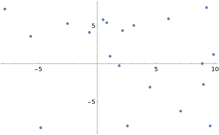
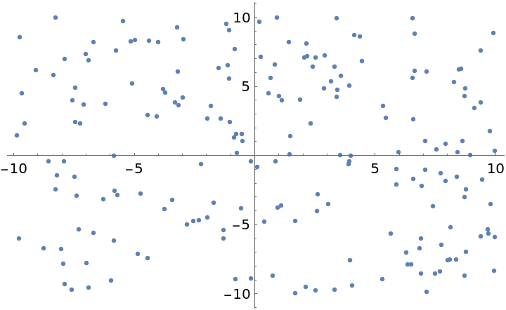
![SeedRandom[1234];
nverts = 200;
ListPlot[pts = RandomReal[{-10, 10}, {nverts, 2}]]](https://www.wolframcloud.com/obj/resourcesystem/images/3d3/3d37845d-6f9c-442b-8de4-6e83503818e7/14c7f94a233ff249.png)
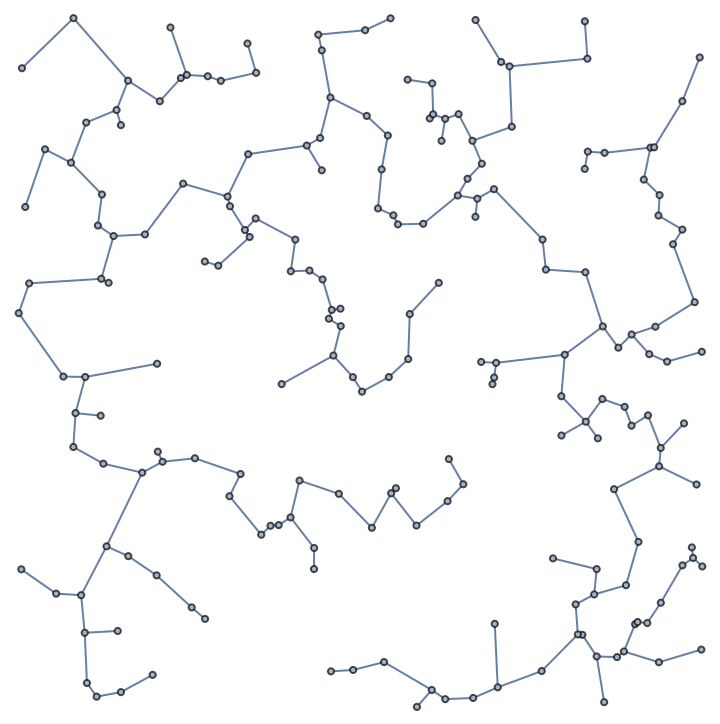
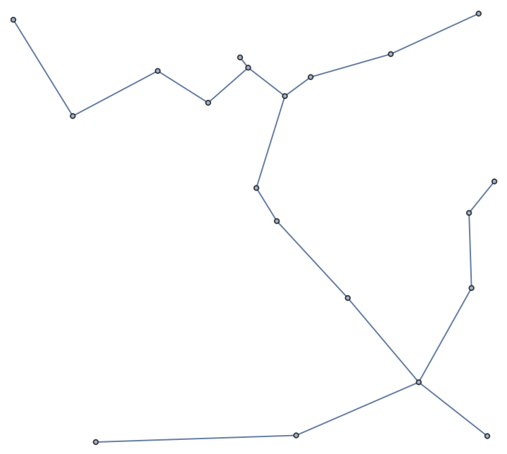
![nverts = 400;
pts = RandomReal[{-10, 10}, {nverts, 2}];
Timing[{tdist, treegraph} = Prim[pts];]](https://www.wolframcloud.com/obj/resourcesystem/images/3d3/3d37845d-6f9c-442b-8de4-6e83503818e7/4734447d71a442d6.png)
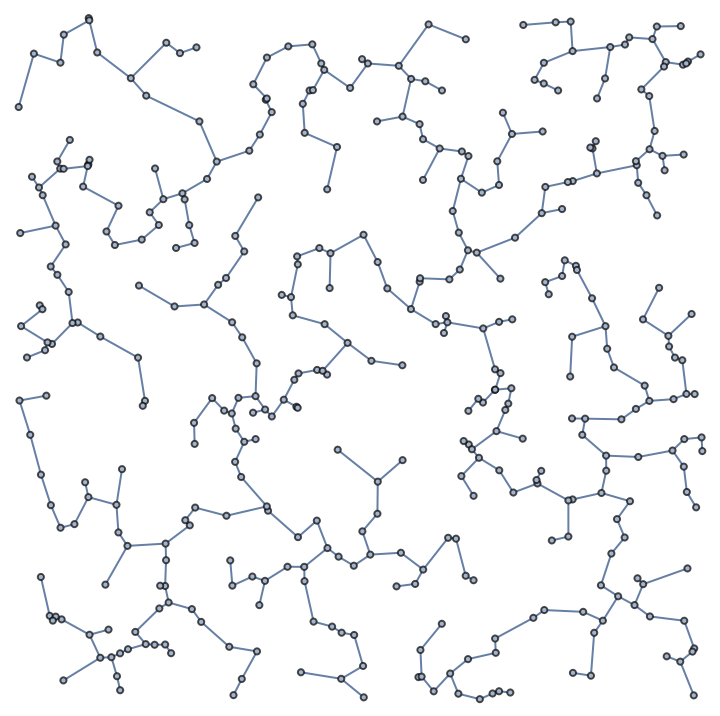
![edges = Flatten[
Table[UndirectedEdge[i, j], {i, nverts - 1}, {j, i + 1, nverts}]];
edgeweights = Flatten[Table[
EuclideanDistance[pts[[i]], pts[[j]]], {i, nverts - 1}, {j, i + 1,
nverts}]];
gr = Graph[Range[nverts], edges, EdgeWeight -> edgeweights, VertexCoordinates -> pts];
Timing[msp = FindSpanningTree[gr, Method -> "Prim"]]](https://www.wolframcloud.com/obj/resourcesystem/images/3d3/3d37845d-6f9c-442b-8de4-6e83503818e7/5e810eea22626696.png)