Wolfram Function Repository
Instant-use add-on functions for the Wolfram Language
Function Repository Resource:
Generate the nth term in the Dyson series of a time-dependent operator
ResourceFunction["DysonTerms"][op,n] generates the order-n term in the Dyson series of the operator op. | |
ResourceFunction["DysonTerms"][op,n,alg] uses operation alg instead of NonCommutativeMultiply. | |
ResourceFunction["DysonTerms"][op,n, alg, t0] uses t0 instead of 0 as the initial integration time. |
| "NumericIntegration" | False | If set as True, it will return a function in terms of NIntegrate where the parameter is the upper limit. Otherwise it will do symbolic integration. |
First order term D1:
| In[1]:= |
| Out[1]= |
Second order term D2:
| In[2]:= |
| Out[2]= |
Second order term with Dot operation:
| In[3]:= |
| Out[3]= |
Third order term D3, with lower integration limit equal to 1:
| In[4]:= |
| Out[4]= |
Dyson series up to third order for some generic operator in 2×2 Pauli algebra:
| In[5]:= |
| Out[5]= |
Get the second order Dyson term for the particular time dependent operator Δ/2 σz + A Cos(ω t) σx:
| In[6]:= | ![ClearAll[h4, \[CapitalDelta], \[Omega], A, \[Sigma]]
h4[t_] := \[CapitalDelta]/2 PauliMatrix[3] + A Cos[\[Omega] t] PauliMatrix[1];
ResourceFunction["DysonTerms"][h4, 2, Dot]](https://www.wolframcloud.com/obj/resourcesystem/images/e85/e85bae31-ac37-418b-841c-a1ae00481fbf/044a2dd08c12f1dd.png) |
| Out[8]= |  |
Consider a time dependent operator for fermionic algebra ![]() , where α and β are time dependent complex valued functions:
, where α and β are time dependent complex valued functions:
| In[9]:= |
Define the algebra:
| In[10]:= | ![alg = NonCommutativeAlgebra[<|
"ScalarVariables" -> Join[Flatten@
Outer[#2[#1] &, {Subscript[\[FormalT], 1], Subscript[\[FormalT], 2]}, {Identity, \[Alpha], \[Beta]}], {\[FormalCapitalT]}]|>];](https://www.wolframcloud.com/obj/resourcesystem/images/e85/e85bae31-ac37-418b-841c-a1ae00481fbf/219709e2f977b9d4.png) |
Function for reducing fermionic algebra {c,c†}=1, {c,c} = 0, {c†,c†} = 0:
| In[11]:= |
Consider the full Dyson series up to the second order:
| In[12]:= |
| Out[12]= |
Normal order the terms; the integrals will depend on the scalar functions α and β:
| In[13]:= |
| Out[13]= |
Define an operator in Pauli algebra:
| In[14]:= |
For a second order term an exact expression could not be obtained or takes too long to integrate:
| In[15]:= |
| Out[15]= |
Get a function to do numeric integration:
| In[16]:= |
Evaluate at some particular final time:
| In[17]:= |
| Out[17]= |
Time dependent drive: VI(t) = g (ⅇⅈ ω t a + ⅇ-ⅈ ω t a†) for bosonic algebra:
| In[18]:= |
Define the algebra and a reduction function:
| In[19]:= |
First order term:
| In[20]:= |
| Out[20]= |
Second order term, simplified in normal order form:
| In[21]:= |
| Out[21]= |  |
| In[22]:= | ![ClearAll[\[CapitalOmega]0, \[Tau], \[Kappa]]
Hchirped[t_] := 1/2 \[CapitalOmega]0 E^(-t^2 / \[Tau]^2) (Cos[\[Kappa] t^2] PauliMatrix[1] + Sin[\[Kappa] t^2] PauliMatrix[2])](https://www.wolframcloud.com/obj/resourcesystem/images/e85/e85bae31-ac37-418b-841c-a1ae00481fbf/1d1c97f146b34289.png) |
Show first order Dyson term to QuantumOperator (using externally the Wolfram Quantum Framework):
| In[23]:= | ![dyson = PacletSymbol[
"Wolfram/QuantumFramework", "Wolfram`QuantumFramework`QuantumOperator"][
1 + PacletSymbol[
"Wolfram/QuantumFramework", "Wolfram`QuantumFramework`QuantumOperator"][ ResourceFunction["DysonTerms"][Hchirped, 1, Dot, -3]], "Parameters" -> {\[CapitalOmega]0, \[Tau], \[Kappa], \[FormalCapitalT]}];](https://www.wolframcloud.com/obj/resourcesystem/images/e85/e85bae31-ac37-418b-841c-a1ae00481fbf/377f75b0e04884f7.png) |
| In[24]:= |
| Out[24]= |  |
Find the Hamiltonian in terms of QuantumOperator:
| In[25]:= | ![(* Evaluate this cell to get the example input *) CloudGet["https://www.wolframcloud.com/obj/01263cf7-4fc9-4d56-abfb-046a8f7d6b31"]](https://www.wolframcloud.com/obj/resourcesystem/images/e85/e85bae31-ac37-418b-841c-a1ae00481fbf/447f7d2b44ac38e9.png) |
Show the first order approximation is good when this value is << 1:
| In[26]:= | ![dysonCondition[\[CapitalOmega]0_, \[Tau]_, \[Kappa]_] := (\[CapitalOmega]0 \[Tau] Sqrt[\[Pi]])/(
2 (1 + \[Kappa]^2 \[Tau]^4)^(1/4))](https://www.wolframcloud.com/obj/resourcesystem/images/e85/e85bae31-ac37-418b-841c-a1ae00481fbf/46b284648519858c.png) |
Case Ω0=1, τ = 1, τ = 10
Use PacletSymbol QuantumEvolve and QuantumState for computing the evolution:
| In[27]:= | ![U = PacletSymbol[
"Wolfram/QuantumFramework", "Wolfram`QuantumFramework`QuantumEvolve"][HchirpedOp[1., 1., 10.],
None, {t, -3, 3}];
\[Psi] = U[
PacletSymbol[
"Wolfram/QuantumFramework", "Wolfram`QuantumFramework`QuantumState"]["+"]];](https://www.wolframcloud.com/obj/resourcesystem/images/e85/e85bae31-ac37-418b-841c-a1ae00481fbf/7e25a984b0b88d5c.png) |
Moderate agreement:
| In[28]:= |
| Out[28]= |
Plot the result from numerically solving the evolution:
| In[29]:= |
| Out[29]= | 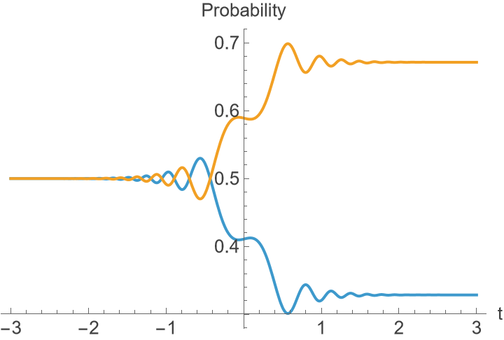 |
Plot result from the Dyson operator:
| In[30]:= | ![Plot[Evaluate[
dyson[1., 1., 10., t][
PacletSymbol[
"Wolfram/QuantumFramework", "Wolfram`QuantumFramework`QuantumState"]["+"]]["Normalize"][
"ProbabilityList"]], {t, -3, 3}, AxesLabel -> {"t", "Probability"},
LabelStyle -> 13]](https://www.wolframcloud.com/obj/resourcesystem/images/e85/e85bae31-ac37-418b-841c-a1ae00481fbf/4067b092d2edcd2a.png) |
| Out[30]= | 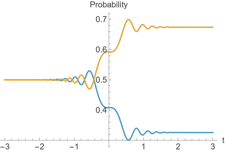 |
Case Ω0=25, τ = 30, τ = 15
Same procedure as the previous case (now we evolve the state |0〉):
| In[31]:= | ![U = PacletSymbol[
"Wolfram/QuantumFramework", "Wolfram`QuantumFramework`QuantumEvolve"][
HchirpedOp[25., 30., 15.], None, {t, -3, 3}];
\[Psi] = U[
PacletSymbol[
"Wolfram/QuantumFramework", "Wolfram`QuantumFramework`QuantumState"]["0"]];](https://www.wolframcloud.com/obj/resourcesystem/images/e85/e85bae31-ac37-418b-841c-a1ae00481fbf/46dbeba6e08f489a.png) |
There will not be good agreement for this case:
| In[32]:= |
| Out[32]= |
Plot the result from numerically solving the evolution:
| In[33]:= |
| Out[33]= | 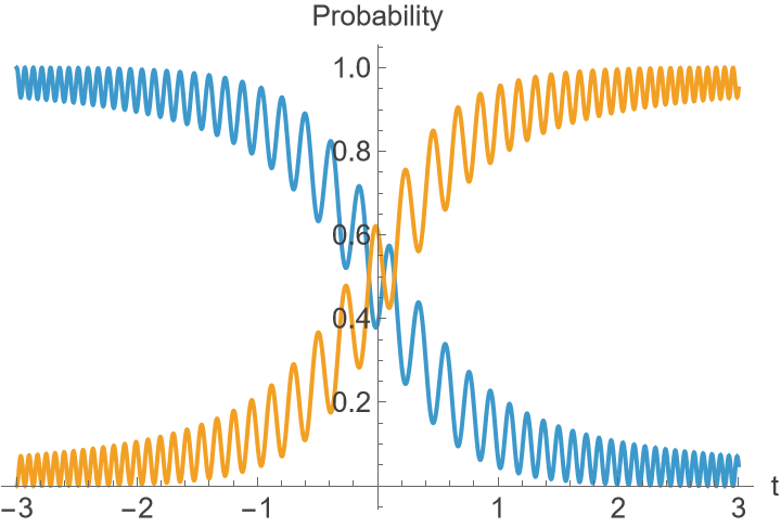 |
Plot result from Dyson:
| In[34]:= | ![Plot[Evaluate[
dyson[25., 30, 15., t][
PacletSymbol[
"Wolfram/QuantumFramework", "Wolfram`QuantumFramework`QuantumState"]["0"]]["Normalize"][
"ProbabilityList"]], {t, -3, 3}, PlotRange -> {0, 1}, AxesLabel -> {"t", "Probability"}, LabelStyle -> 13]](https://www.wolframcloud.com/obj/resourcesystem/images/e85/e85bae31-ac37-418b-841c-a1ae00481fbf/1e3361496a58a552.png) |
| Out[34]= |  |
Load the function for computing terms of Magnus expansion:
| In[35]:= |
| Out[35]= |
For the first order term D1=Ω1 they have the same form:
| In[36]:= |
| Out[36]= |
Second order Dyson term expressed in terms of Magnus terms ![]() :
:
| In[37]:= | ![MagnusTerms[\[FormalCapitalB], 2, "TimeIntegration" -> True] + 1/2 MagnusTerms[\[FormalCapitalB], 1, "TimeIntegration" -> True] ** MagnusTerms[\[FormalCapitalB], 1, "TimeIntegration" -> True]](https://www.wolframcloud.com/obj/resourcesystem/images/e85/e85bae31-ac37-418b-841c-a1ae00481fbf/68650ead31361785.png) |
| Out[37]= |
For the second order Dyson term, it is not trivial to see they are equal:
| In[38]:= | ![ResourceFunction["DysonTerms"][\[FormalCapitalB], 2]/(-I)^2](https://www.wolframcloud.com/obj/resourcesystem/images/e85/e85bae31-ac37-418b-841c-a1ae00481fbf/671e2b4f071f786d.png) |
| Out[38]= |
Define a time dependent operator in the Pauli basis:
| In[39]:= |
Result from Dyson:
| In[40]:= | ![res1 = ResourceFunction["DysonTerms"][h1, 2, Dot]/(-I)^2;](https://www.wolframcloud.com/obj/resourcesystem/images/e85/e85bae31-ac37-418b-841c-a1ae00481fbf/61edcdb8642df59c.png) |
Result from Magnus:
| In[41]:= | ![res2 = MagnusTerms[h1, 2, Dot, "TimeIntegration" -> True] + 1/2 MagnusTerms[h1, 1, Dot, "TimeIntegration" -> True] . MagnusTerms[h1, 1, Dot, "TimeIntegration" -> True];](https://www.wolframcloud.com/obj/resourcesystem/images/e85/e85bae31-ac37-418b-841c-a1ae00481fbf/24656323efe9c193.png) |
| In[42]:= |
| Out[42]= |
Dyson third order term:
| In[43]:= | ![res1 = ResourceFunction["DysonTerms"][h1, 3, Dot]/(-I)^3;](https://www.wolframcloud.com/obj/resourcesystem/images/e85/e85bae31-ac37-418b-841c-a1ae00481fbf/56fe0799217c6298.png) |
![]()
| In[44]:= | ![res2 = With[{\[CapitalOmega]1 = MagnusTerms[h1, 1, Dot, "TimeIntegration" -> True], \[CapitalOmega]2 = MagnusTerms[h1, 2, Dot, "TimeIntegration" -> True], \[CapitalOmega]3 = MagnusTerms[h1, 3, Dot, "TimeIntegration" -> True]},
\[CapitalOmega]3 + 1/2 (\[CapitalOmega]1 . \[CapitalOmega]2 + \[CapitalOmega]2 . \[CapitalOmega]1) + 1/6 \[CapitalOmega]1 . \[CapitalOmega]1 . \[CapitalOmega]1];](https://www.wolframcloud.com/obj/resourcesystem/images/e85/e85bae31-ac37-418b-841c-a1ae00481fbf/2e8afd757f02eae5.png) |
| In[45]:= |
| Out[45]= |
For the fourth term we have ![]() +
+ ![]() .
In general, a Dyson term is generated by the non-commutative products of Magnus terms of the corresponding order, with a 1/n! factor introduced by the number of terms in that product.
.
In general, a Dyson term is generated by the non-commutative products of Magnus terms of the corresponding order, with a 1/n! factor introduced by the number of terms in that product.
If supplying an algebraic operation, it has to be one compatible with NonCommutativeAlgebra:
| In[46]:= |
| Out[46]= |
However it is possible to enforce a desired operation by defining a custom algebra:
| In[47]:= |
| Out[48]= |
This work is licensed under a Creative Commons Attribution 4.0 International License