Basic Examples (2) 

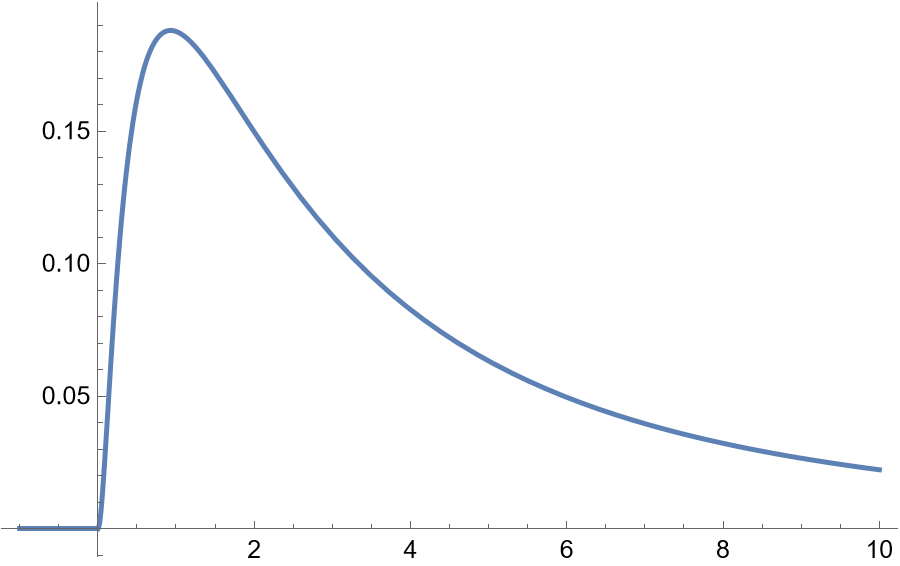
In this example, plotting the density, the right tail exponent has a heavy power tail with tail exponent 1.5, the left tail exponent at 3.0 mainly controls the shape of the left side of the distribution and does not contribute to left tail behavior:

In[1]:=

Out[1]=

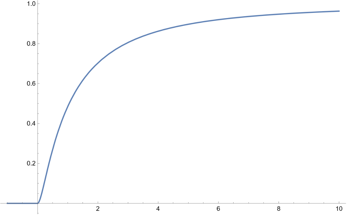
The mean cannot be expressed as a simple function of parameters. It will exist when the right tail exponent, α is greater than 1. Numerical integration provides a solution:

In[2]:=

Out[2]=

The variance for this set of parameters does not exist because α is less than 2, making this a heavy-tailed distribution:

In[3]:=

Out[3]=

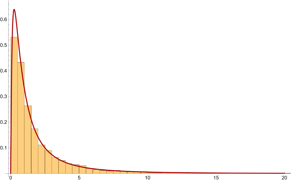
Generate a random sample for the DoubleParetoLogNormalDistributon with a right Pareto tail exponent of 1.8 and a left tail exponent of 2. The PDF and histogram are shown as well as the parameter estimates from the sample, s. Note that a short form name for the distribution is available in the definition:

In[4]:=

Out[8]=

The estimated distribution with parameters can be computed with the function EstimatedDistribution:

In[9]:=

Out[9]=

The parameters are listed with the function FindDistributionParameters; α is the right tail exponent, β the left tail exponent, μ a location parameter, σ the scale parameter:

In[10]:=

Out[10]=

Scope (3) 

Here is a plot of the continuous distribution function:

In[11]:=

Out[11]=

The Quantile function uses FindRoot and CDF and is listable, but slow:

In[12]:=

Out[12]=

The function DistributionParameterAssumptions shows the domain of each parameter:

In[13]:=

Out[13]=

Applications (3) 

The Log[high/low] of a intraday stock market price can be used as a surrogate measure of daily volatility. This measure has a distribution which is well fit by the DoubleParetoLogNormalDistribution:

In[14]:=

Out[13]=

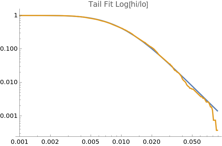
This LogLogPlot shows the right tail behavior of the estimated distribution from the data and the distribution fit. The tail behavior becomes log-log linear consistent with a power tail distribution:

In[15]:=

Out[16]=

Results from hypothesis testing:

In[17]:=

Out[18]=

Properties and Relations (10) 

The distribution can be efficiently derived using TransformedDistribution and ParameterMixtureDistribution as shown below. ALD is an asymmetric Laplace distribution with a right tail parameter, α, and a left tail parameter, β, centered at zero. The DoubleParetoLogNormalDistribution can then be described as a parameter mixture distribution of the LogNormalDistribution, with the location parameter determined by ALD:

In[19]:=

Out[19]=

The DoubleParetoLogNormalDistribution then can be considered a mixture of the ALD and a LogNormalDistribution:

In[20]:=

Out[20]=

In[21]:=

Out[21]=

The densities are the same:

In[22]:=

Out[22]=

The normal Laplace distribution (see resource function NormalLaplaceDistribution) can be derived as the distribution of the difference between two exponentials plus a normal random variable, i.e. it represents the sum of an ALD random variable and a normal random variable:

In[23]:=

Out[23]=

The PDF of the transformed distribution:

In[24]:=

Out[24]=

Generate the NormalLaplaceDistribution:

In[25]:=

Out[25]=

The density formulas are equal:

In[26]:=

Out[26]=

TransformedDistribution does not expand the NormalLaplaceDistribution into basic components and cannot be used directly to solve the relationship to the DoubleParetoLogNormalDistribution:

In[27]:=

Out[27]=

The basic components of the the NormalLaplaceDistribution are exponentiated to give the TransformedDistribution form of the DoubleParetoLogNormalDistribution:

In[28]:=

Out[28]=

FullSimplify can find the equality (this may take several minutes):

In[29]:=

Out[29]=