Function Repository Resource:

DiscreteHartleyTransform

Source Notebook

Compute the discrete Hartley transform of a list

Contributed by: Jan Mangaldan

ResourceFunction["DiscreteHartleyTransform"][list]

computes the discrete Hartley transform of a list of complex numbers.

Details

The discrete Hartley transform vs of a list ur of length n is defined to be . The normalization is chosen such that the transform is its own inverse.
The discrete Hartley transform is sometimes defined to have the normalization constant 1 or instead.
The discrete Hartley transform is real-valued for real-valued data.
The list of data supplied to ResourceFunction["DiscreteHartleyTransform"] need not have a length equal to a power of two.
The list given in ResourceFunction["DiscreteHartleyTransform"][list] can be nested to represent an array of data in any number of dimensions.
The array of data must be rectangular.
If the elements of list are exact numbers, ResourceFunction["DiscreteHartleyTransform"] begins by applying N to them.
ResourceFunction["DiscreteHartleyTransform"] can be used on SparseArray objects.

Examples

Basic Examples (1) 

Compute a discrete Hartley transform:

In[1]:=
ResourceFunction["DiscreteHartleyTransform"][{1, 1, 2, 2, 1, 1, 0, 0}]
Out[1]=

Scope (4) 

x is a list of real values:

In[2]:=
x = {1, 0, 0, 1, 0, 0, 1};

Compute the Hartley transform with machine arithmetic:

In[3]:=
ResourceFunction["DiscreteHartleyTransform"][x]
Out[3]=

Compute using 24-digit precision arithmetic:

In[4]:=
ResourceFunction["DiscreteHartleyTransform"][N[x, 24]]
Out[4]=

Compute a complex Hartley transform:

In[5]:=
v = RandomComplex[1 + I, 17];
In[6]:=
ResourceFunction["DiscreteHartleyTransform"][v]
Out[6]=

This is equivalent to separately taking the Hartley transforms of the real and imaginary parts:

In[7]:=
ResourceFunction["DiscreteHartleyTransform"][Re[v]] + I ResourceFunction["DiscreteHartleyTransform"][Im[v]]
Out[7]=

Compute a 2D Hartley transform:

In[8]:=
ResourceFunction["DiscreteHartleyTransform"][
 RandomReal[{-1, 1}, {3, 6}]]
Out[8]=

x is a rank 3 tensor with nonzero diagonal:

In[9]:=
x = ConstantArray[0, {2, 3, 4}]; x[[1, 1, 1]] = 1; x[[2, 2, 2]] = 1;

Compute the 3D Hartley transform:

In[10]:=
ResourceFunction["DiscreteHartleyTransform"][x]
Out[10]=

Applications (2) 

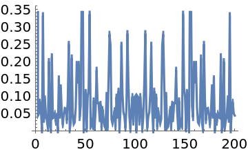
Use the discrete Hartley transform to compute the power spectrum of "white noise":

In[11]:=
dat = RandomReal[1, 200];
fht = ResourceFunction["DiscreteHartleyTransform"][dat];
ListLinePlot[(fht^2 + RotateRight[Reverse[fht]]^2)/2]
Out[14]=

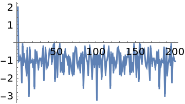
Show the logarithmic spectrum, including the first (DC) component:

In[15]:=
ListLinePlot[Log10[fht^2 + RotateRight[Reverse[fht]]^2], PlotRange -> All]
Out[25]=

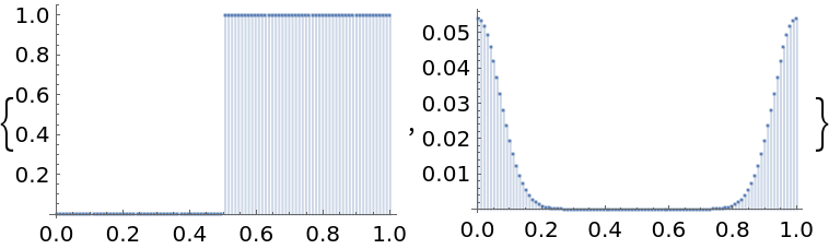
Compute discrete cyclic convolutions to smooth a discontinuous function with a Gaussian:

In[26]:=
n = 100; dx = 1./(n - 1);
a = Table[UnitStep[x - 1/2], {x, 0, 1, dx}];
b = Table[
   If[x <= 1/2, Exp[-100 x^2], Exp[-100 (1 - x)^2]], {x, 0, 1, dx}];
b = b/Total[b];
In[27]:=
{ListPlot[a, Filling -> Axis, DataRange -> {0, 1}], ListPlot[b, Filling -> Axis, PlotRange -> All, DataRange -> {0, 1}]}
Out[27]=

Compute the cyclic convolution:

In[28]:=
(* Evaluate this cell to get the example input *) CloudGet["https://www.wolframcloud.com/obj/711d418b-94f5-4d5a-b950-71d8b55c74c6"]

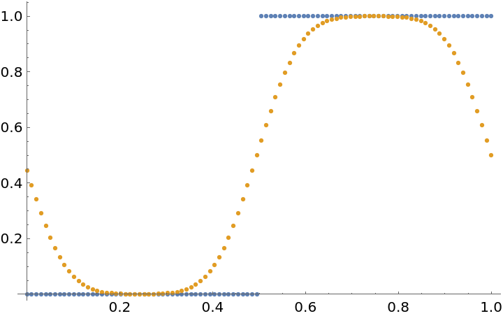
Show the original and smoothed function:

In[29]:=
ListPlot[{a, c}, DataRange -> {0, 1}]
Out[29]=

The convolution is consistent with ListConvolve:

In[30]:=
Max[Abs[c - ListConvolve[a, b, {1, 1}]]]
Out[30]=

Properties and Relations (4) 

Compute the discrete Hartley transform from its definition:

In[31]:=
u = N[{1, 2, 3, 4, 5, 6, 7}];
n = Length[u];
In[32]:=
AbsoluteTiming[v1 = Table[1/Sqrt[n] \!\(TraditionalForm\`
\*UnderoverscriptBox[\(\[Sum]\), \(r = 1\), \(n\)]\*
TemplateBox[{"u", "r"},
"IndexedDefault"]\ \((Cos[
\*FractionBox[\(2  \[Pi]\ \((r - 1)\)\ \((s - 1)\)\), \(n\)]] + Sin[
\*FractionBox[\(2  \[Pi]\ \((r - 1)\)\ \((s - 1)\)\), \(n\)]])\)\), {s, 1, n}]]
Out[32]=

DiscreteHartleyTransform is faster:

In[33]:=
AbsoluteTiming[v2 = ResourceFunction["DiscreteHartleyTransform"][u]]
Out[33]=
In[34]:=
Chop[v1 - v2]
Out[34]=

Compute the discrete Hartley transform of a vector by multiplying it with the Hartley matrix:

In[35]:=
u = N[{1, 2, 3, 4, 5, 6, 7}];
n = Length[u];
In[36]:=
AbsoluteTiming[v1 = ResourceFunction["HartleyMatrix"][n] . u]
Out[36]=

DiscreteHartleyTransform is faster:

In[37]:=
AbsoluteTiming[v2 = ResourceFunction["DiscreteHartleyTransform"][u]]
Out[37]=
In[38]:=
Chop[v1 - v2]
Out[38]=

The discrete Hartley transform is its own inverse:

In[39]:=
v = RandomReal[{-2, 2}, 13];
In[40]:=
v - ResourceFunction["DiscreteHartleyTransform"][
   ResourceFunction["DiscreteHartleyTransform"][v]] // Chop
Out[40]=

A list of numbers:

In[41]:=
v = RandomReal[{-2, 2}, 13];

Compute its discrete Hartley transform:

In[42]:=
fht = ResourceFunction["DiscreteHartleyTransform"][v]
Out[42]=

Use the discrete Hartley transform to compute the discrete Fourier transform:

In[43]:=
rev = RotateRight[Reverse[fht]];
(fht + rev)/2 + I (fht - rev)/2
Out[44]=

Compare with the result of Fourier:

In[45]:=
Fourier[v]
Out[45]=

Version History

  • 1.1.0 – 13 March 2023
  • 1.0.0 – 13 February 2023

Source Metadata

Related Resources

License Information