Function Repository Resource:

SymbolicFourier

Source Notebook

A symbolic version of the Fourier function

Contributed by: Jan Mangaldan

ResourceFunction["SymbolicFourier"][list]

finds the discrete Fourier transform of a list of complex numbers.

Details and Options

The discrete Fourier transform vs of a list ur of length n is by default defined to be .
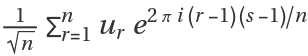
As with the numeric Fourier function, the zero frequency term appears at position 1 in the resulting list.
Other definitions are used in some scientific and technical fields.
Different choices of definitions can be specified using the option FourierParameters.
With the setting FourierParameters{a,b}, the discrete Fourier transform computed by Fourier is .
Some common choices for {a,b} are {0,1} (default), {-1,1} (data analysis) and {1,-1} (signal processing).
The setting b=-1 effectively corresponds to conjugating both input and output lists.
To ensure a unique inverse discrete Fourier transform, |b| must be relatively prime to n.
The list of data supplied to ResourceFunction["SymbolicFourier"] need not have a length equal to a power of two.
The list given in ResourceFunction["SymbolicFourier"][list] can be nested to represent an array of data in any number of dimensions, and does not need to have numeric entries.
The array of data must be rectangular.

Examples

Basic Examples (2) 

Find a discrete Fourier transform:

In[1]:=
ResourceFunction["SymbolicFourier"][{1, 1, 2, 2, 1, 1, 0, 0}]
Out[1]=

Compare with the built-in Fourier:

In[2]:=
{N[%], Fourier[N[{1, 1, 2, 2, 1, 1, 0, 0}]]} // Chop
Out[2]=

Scope (3) 

SymbolicFourier can be used on lists with symbolic elements:

In[3]:=
ResourceFunction["SymbolicFourier"][Array[\[FormalX], 5]]
Out[3]=

Compute the 2D Fourier transform of a symbolic 2×2 matrix:

In[4]:=
ResourceFunction["SymbolicFourier"][{{a, b}, {c, d}}]
Out[4]=

Compute the 2D Fourier transform of a section of the Hilbert matrix:

In[5]:=
ResourceFunction["SymbolicFourier"][HilbertMatrix[{2, 3}]]
Out[5]=

x is a rank-3 tensor with nonzero diagonal:

In[6]:=
x = ConstantArray[0, {2, 3, 4}]; x[[1, 1, 1]] = 1; x[[2, 2, 2]] = 1;

Compute the 3D Fourier transform:

In[7]:=
ResourceFunction["SymbolicFourier"][x]
Out[7]=

Options (1) 

FourierParameters (1) 

Use FourierParameters to specify a different normalization:

In[8]:=
ResourceFunction["SymbolicFourier"][Array[\[FormalX], 5], FourierParameters -> {1, -1}]
Out[8]=

Properties and Relations (2) 

Applying SymbolicFourier to a vector is the same as pre-multiplying the vector with FourierMatrix:

In[9]:=
r1 = ResourceFunction["SymbolicFourier"][Array[\[FormalX], 6]]
Out[9]=
In[10]:=
r2 = FourierMatrix[6] . Array[\[FormalX], 6]
Out[10]=
In[11]:=
r1 == r2 // FullSimplify
Out[11]=

The result of SymbolicFourier produces a result in factored form, often with a lower LeafCount:

In[12]:=
{LeafCount[r1], LeafCount[r2]}
Out[12]=

Version History

  • 1.1.0 – 06 March 2023
  • 1.0.0 – 26 May 2021

Source Metadata

Related Resources

License Information