Options (34)
AxesLabel (1)
Specify labels for the x- and y-axes:
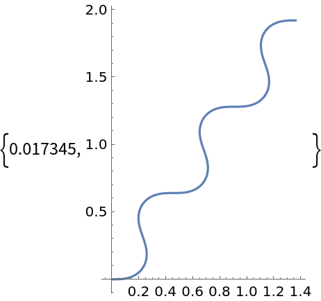
AxesOrigin (2)
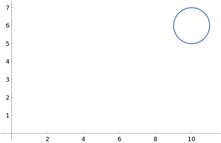
Determine where the axes cross automatically:
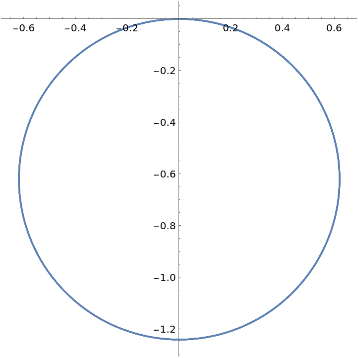
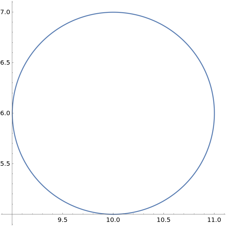
Specify the axes origin at the point {0,0}:
ColorFunction (5)
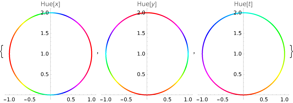
Color the curve by scaled x-, y- or t-values:
Use a named color gradient:
ColorFunction has higher priority than PlotStyle:
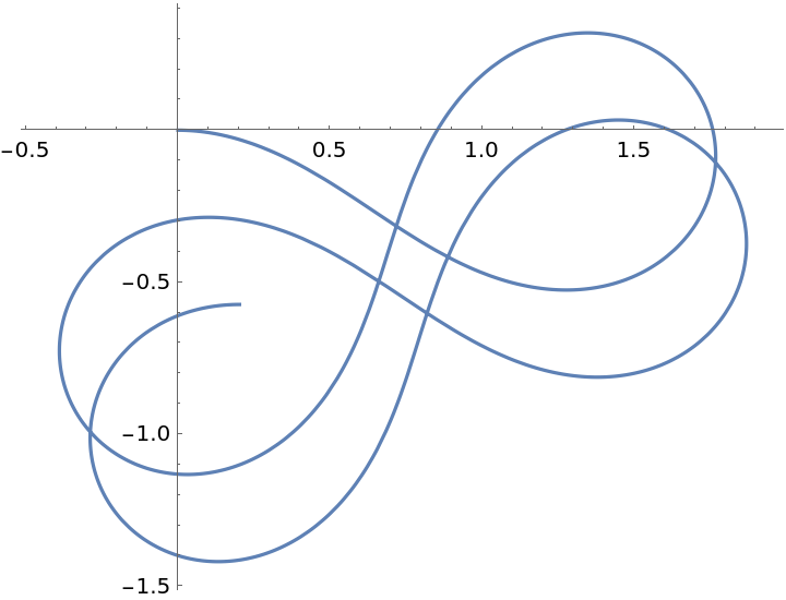
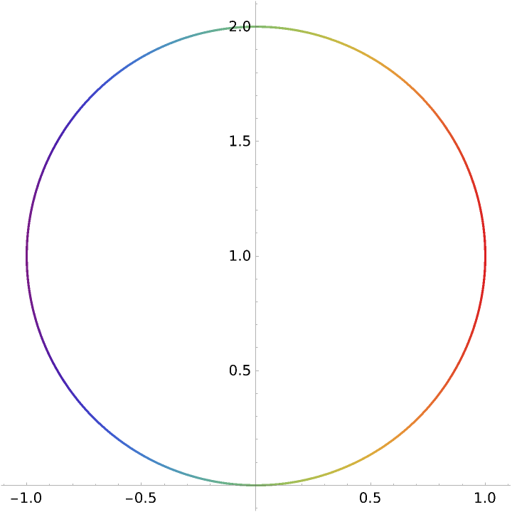
Use red for the parameter t>2π:
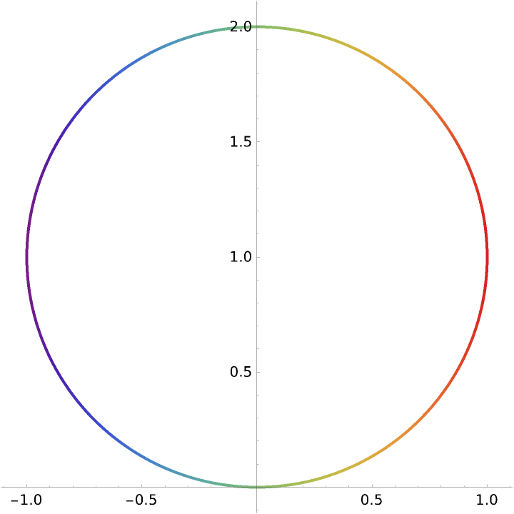
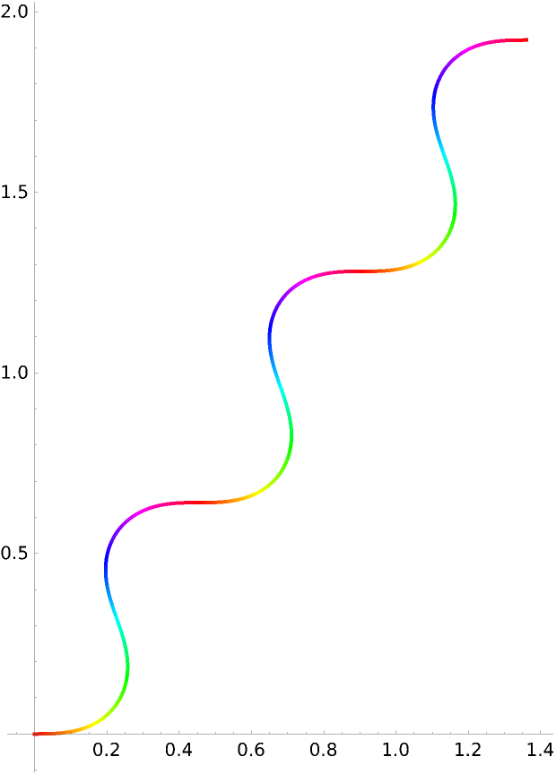
Color by the absolute curvature:
ColorFunctionScaling (1)
Color the curve by the phase of the sine:
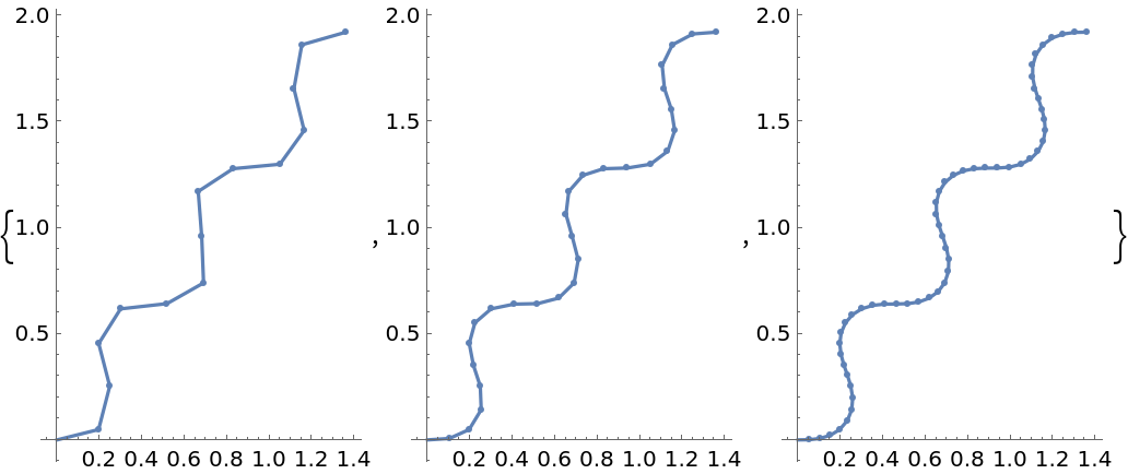
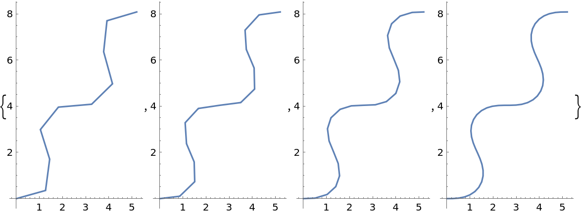
MaxRecursion (1)
Each level of MaxRecursion will adaptively subdivide the initial mesh into a finer mesh:
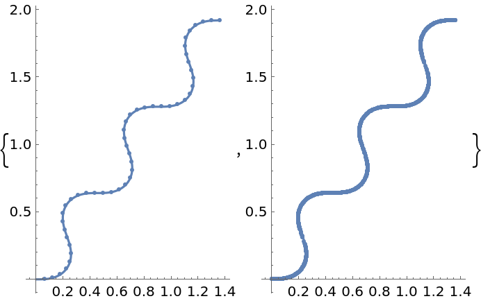
Mesh (1)
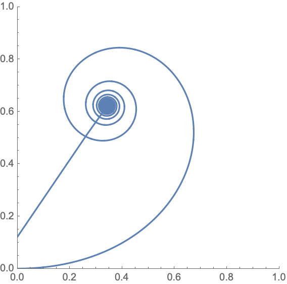
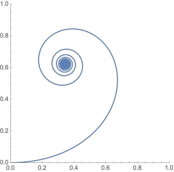
Show the initial and final sampling meshes:
PerformanceGoal (2)
Generate a higher-quality plot:
Emphasize performance, possibly at the cost of quality:
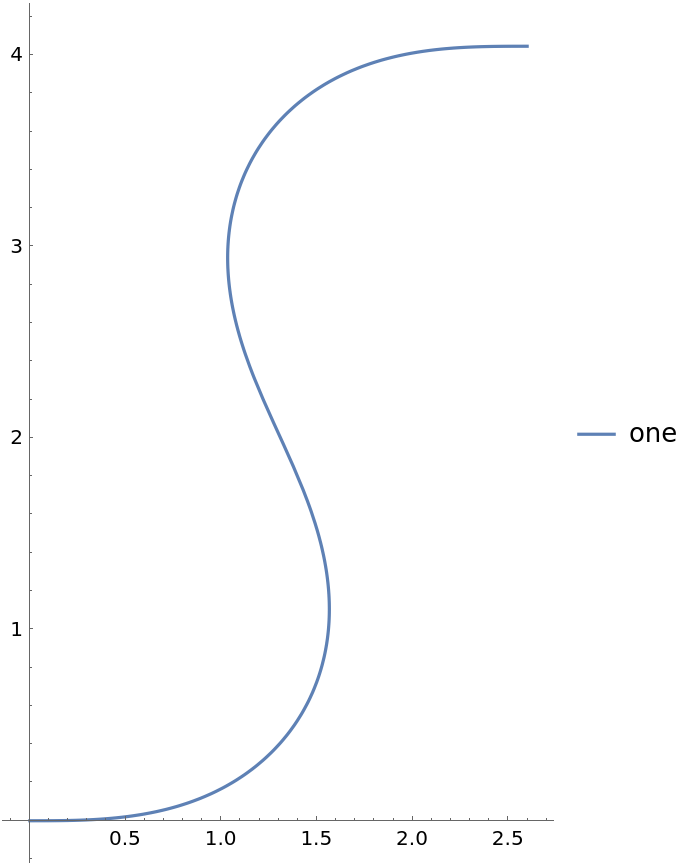
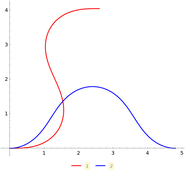
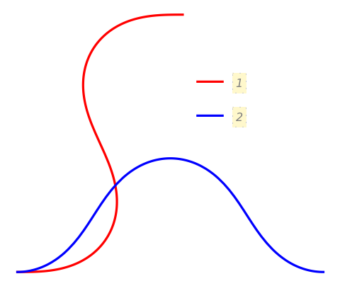
PlotLabels (5)
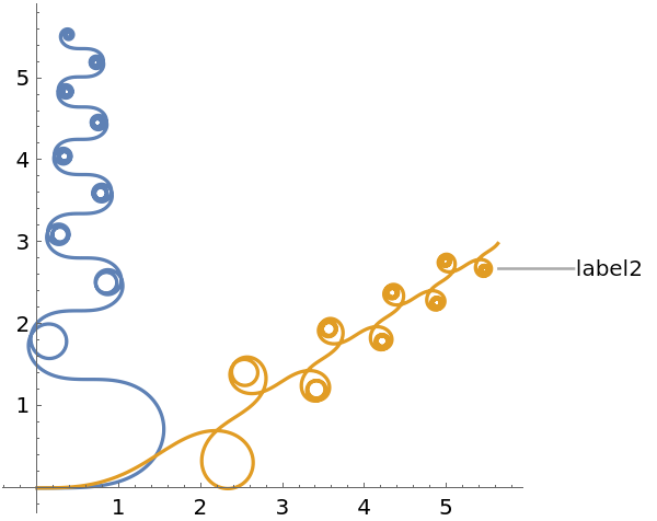
Specify the text to label the curves:
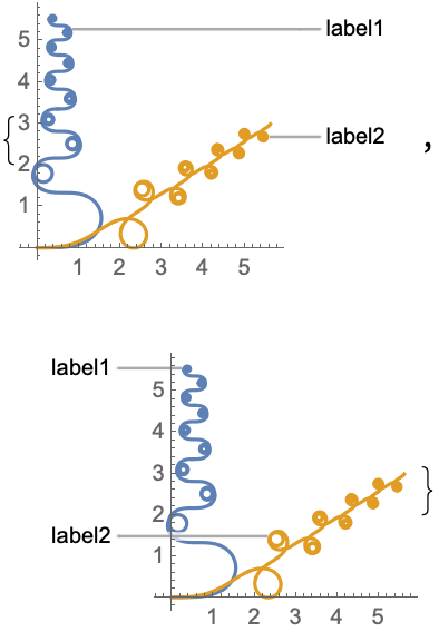
Place the labels above the curves:
Place the labels differently for each curve:
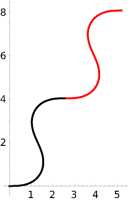
Use callouts to identify the curves:
Put labels relative to the outside of the curves:
Use None to not add a label:
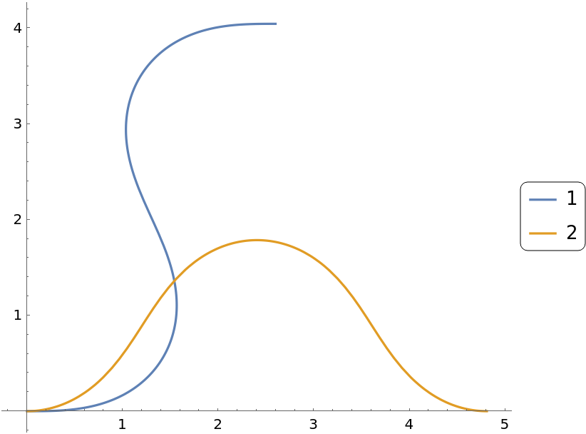
PlotLegends (5)
No legends are used by default:
Create a legend with specific labels:
PlotLegends picks up PlotStyle values automatically:
Use Placed to position legends:
Place legends inside:
Use LineLegend to modify the appearance of the legend:
PlotPoints (1)
Use more initial points to get a smoother plot:
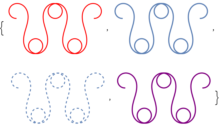
PlotStyle (3)
Use different style directives:
By default, different styles are chosen for multiple curves:
Explicitly specify the style for different curves:
PlotTheme (1)
Use a marketing theme:
WorkingPrecision (2)
Evaluate functions using machine-precision arithmetic:
Evaluate functions using arbitrary-precision arithmetic:
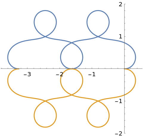
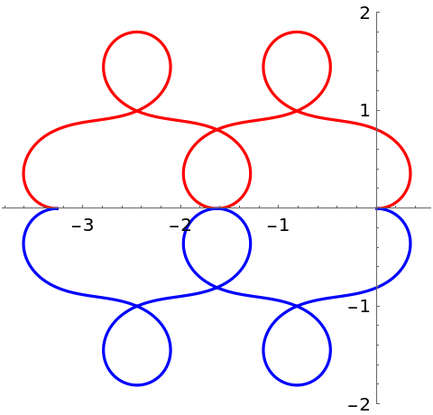
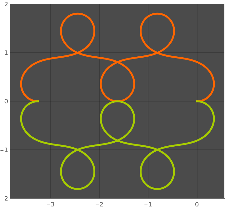
Neat Examples (4)
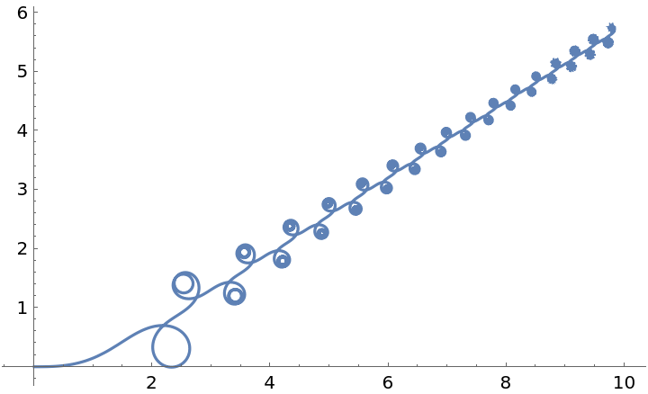
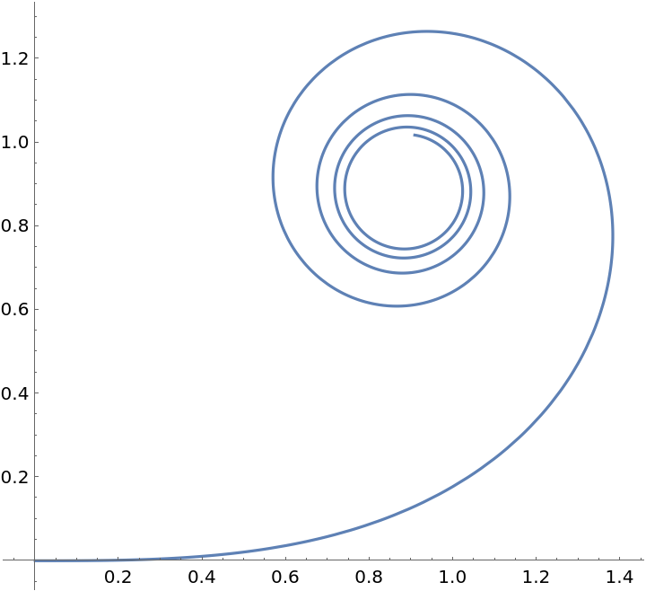
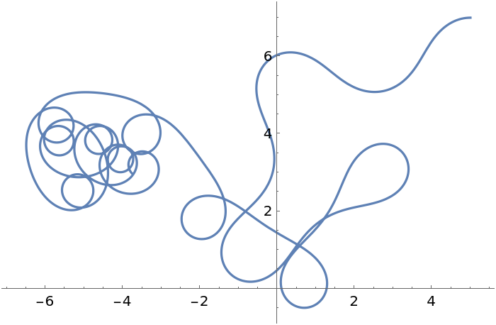
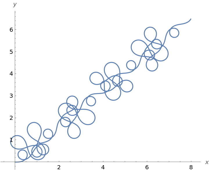
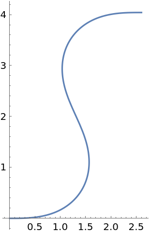
Plot an increasingly-curvy curve:
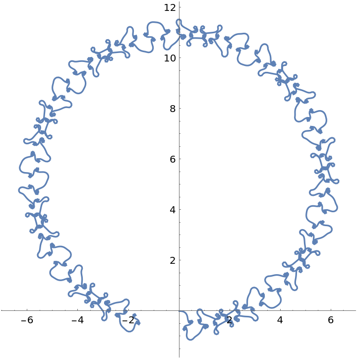
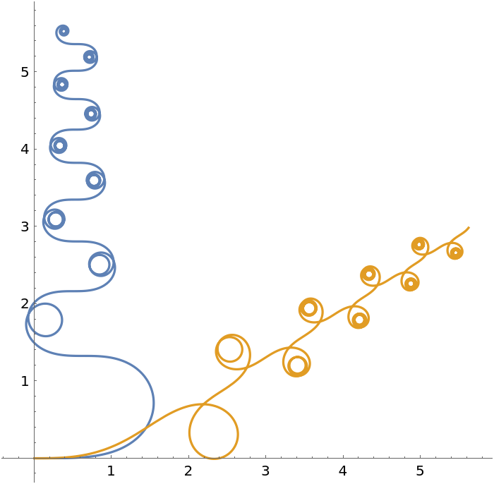
Elementary function can lead to very complicated patterns:
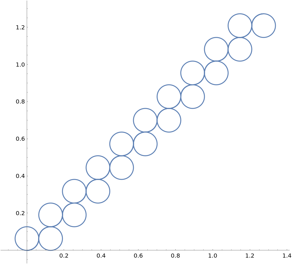
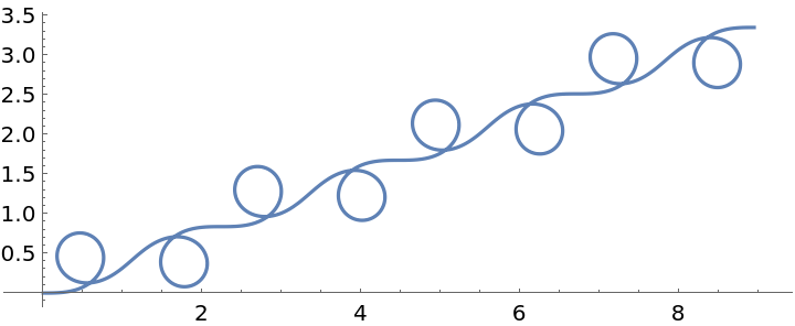
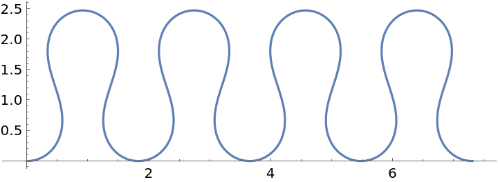
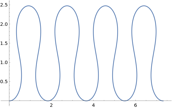
Plot a bunch of connected circles:
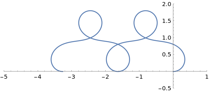
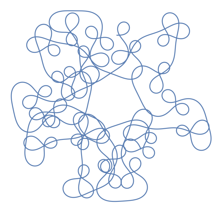
Create intricate non-repeating patterns:
![Table[ResourceFunction["CurvaturePlot"][1, {t, 0, 2 Pi}, ColorFunction -> Function[{x, y, t}, i], PlotLabel -> i, PlotStyle -> Thick], {i, {Hue[x], Hue[y], Hue[t]}}]](https://www.wolframcloud.com/obj/resourcesystem/images/bd7/bd70ad64-1171-45cf-b64b-16d211033eb5/70350fe95689c5a6.png)
![ResourceFunction["CurvaturePlot"][
0.65 Pi Cos[t], {t, 0, 8 Pi}, {{10, 10}, Pi/4}, PlotRange -> All, ImageSize -> 350, ColorFunction -> Function[{x, y, t}, ColorData[{"Rainbow", {0, 0.65 Pi}}][0.65 Pi Abs@Cos[t]]], ColorFunctionScaling -> False]](https://www.wolframcloud.com/obj/resourcesystem/images/bd7/bd70ad64-1171-45cf-b64b-16d211033eb5/7c78d3580832cdc7.png)
![Table[ResourceFunction["CurvaturePlot"][6 Sin[2 Pi t], {t, 0, 3}, MaxRecursion -> i, PlotPoints -> 15, Mesh -> All], {i, 0, 2}]](https://www.wolframcloud.com/obj/resourcesystem/images/bd7/bd70ad64-1171-45cf-b64b-16d211033eb5/5be7584cf24fe28b.png)
![{ResourceFunction["CurvaturePlot"][6 Sin[2 Pi t], {t, 0, 3}, Mesh -> Full], ResourceFunction["CurvaturePlot"][6 Sin[2 Pi t], {t, 0, 3}, Mesh -> All]}](https://www.wolframcloud.com/obj/resourcesystem/images/bd7/bd70ad64-1171-45cf-b64b-16d211033eb5/4bab2108517bb726.png)
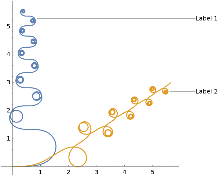
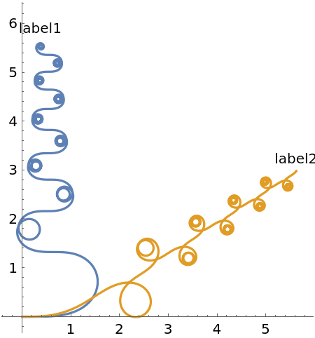
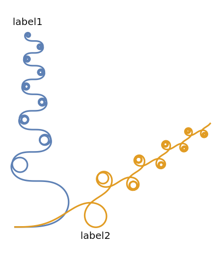
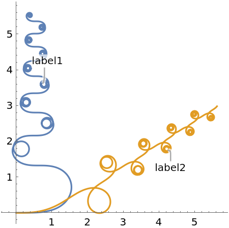
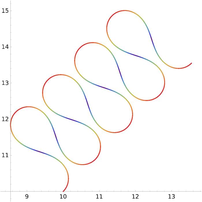
![Table[ResourceFunction[
"CurvaturePlot"][{Sin[t] t, Cos[t] t}, {t, 0, 30}, PlotLabels -> Callout[{"label1", "label2"}, pos]], {pos, {After, Before}}]](https://www.wolframcloud.com/obj/resourcesystem/images/bd7/bd70ad64-1171-45cf-b64b-16d211033eb5/2fbdd4eb5c1a2a70.png)

![Table[ResourceFunction["CurvaturePlot"][5 Cos[t], {t, 0, 4 Pi}, PlotStyle -> ps, Axes -> False], {ps, {Red, Thick, Dashed, Directive[Purple, Thick]}}]](https://www.wolframcloud.com/obj/resourcesystem/images/bd7/bd70ad64-1171-45cf-b64b-16d211033eb5/7acfe0027cf6c768.png)