Wolfram Function Repository
Instant-use add-on functions for the Wolfram Language
Function Repository Resource:
Plot a curve defined by its curvature and torsion
ResourceFunction["CurvatureTorsionPlot3D"][{κ,τ},{t,tmin,tmax},{a0,p,q,r}] plots the curve c defined by its curvature κ and torsion τ, written as functions of t and having initial conditions c(a0)=p,c'(a0)=q and c''(a0)=κ(a0)r. | |
ResourceFunction["CurvatureTorsionPlot3D"][{κ,τ},{t,tmin,tmax}] plots the curve using default initial conditions. | |
ResourceFunction["CurvatureTorsionPlot3D"][{{κ1,τ1},…},{t,tmin,tmax}] plots several curves defined by their curvatures κi and torsions τi. |
Zero torsion gives a plane curve:
| In[1]:= |
| Out[1]= | 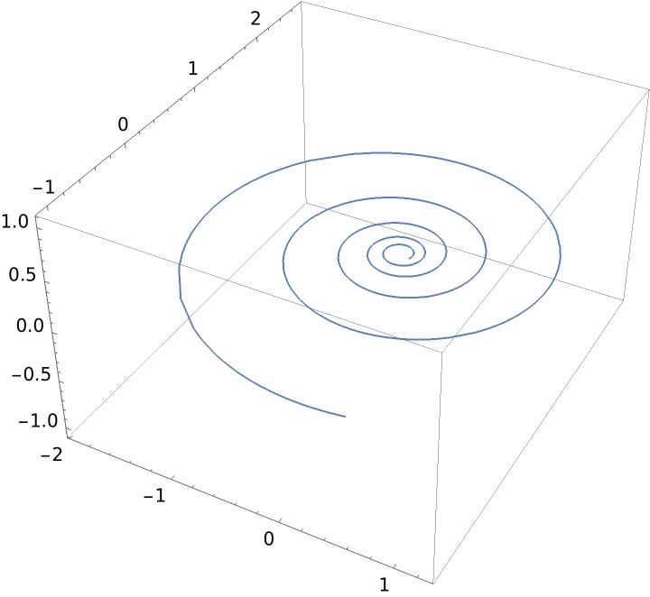 |
Constant curvature and torsion gives a helix:
| In[2]:= |
| Out[2]= | 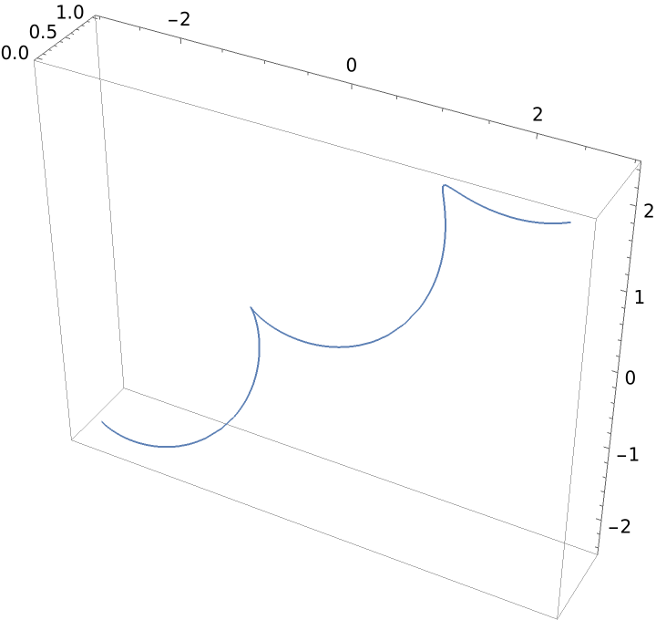 |
Linear curvature and constant torsion:
| In[3]:= |
| Out[3]= | 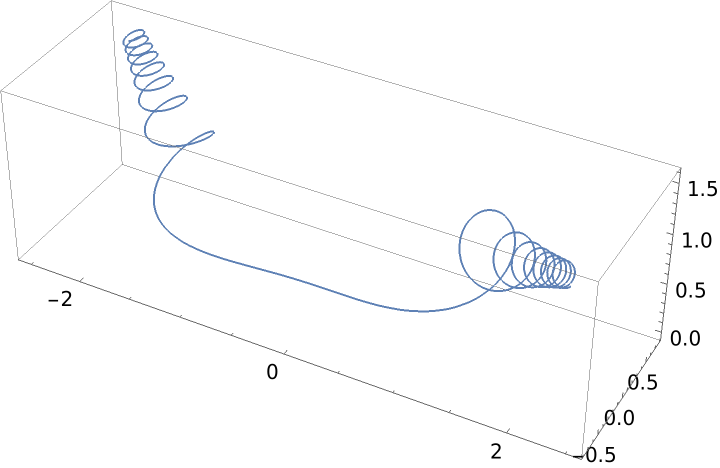 |
Linear curvature and torsion:
| In[4]:= |
| Out[4]= | 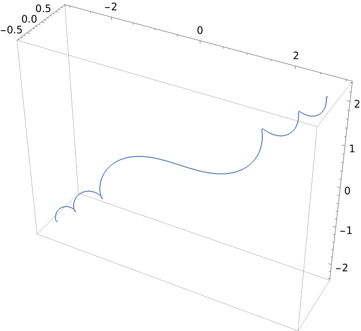 |
Constant curvature and linear torsion:
| In[5]:= |
| Out[5]= | 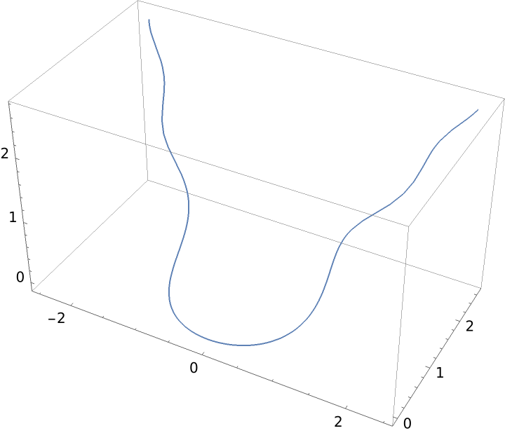 |
Constant curvature and sinusoidal torsion:
| In[6]:= |
| Out[6]= | 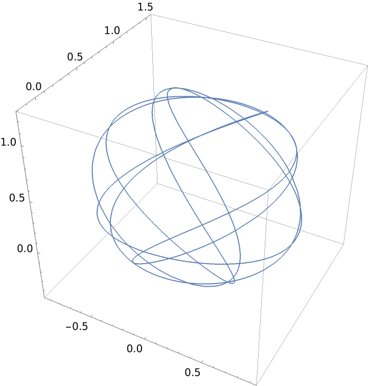 |
Sine-cosine curvature and torsion:
| In[7]:= |
| Out[7]= | 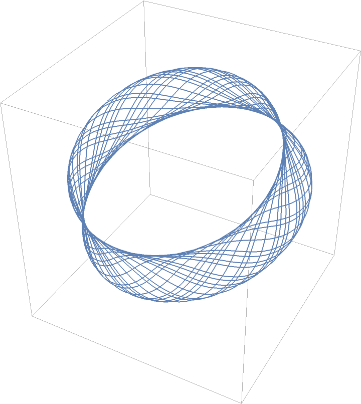 |
Using a sawtooth wave curve:
| In[8]:= |
| Out[8]= | 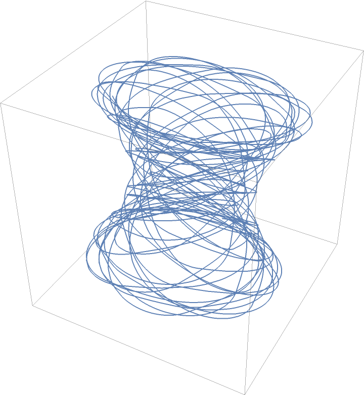 |
Increasing torsion ends in a closed curve:
| In[9]:= | ![Partition[
Table[ResourceFunction[
"CurvatureTorsionPlot3D"][{1, 1/12 n Sin[t]}, {t, 0, 4 \[Pi]}, Axes -> None, Boxed -> False, ViewPoint -> {1, 1, 2}], {n, 12}], 4] // GraphicsGrid](https://www.wolframcloud.com/obj/resourcesystem/images/30b/30b9ee64-cce4-4218-ac05-21db0809f21b/11a3e64c4625e853.png) |
| Out[9]= | 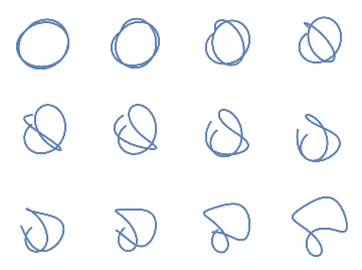 |
All graphics together:
| In[10]:= | ![ResourceFunction["CurvatureTorsionPlot3D"][
Table[{1, 1/12 n Sin[t]}, {n, 12}], {t, 0, 4 \[Pi]}, Axes -> None, Boxed -> False, ViewPoint -> {1, 1, 2}]](https://www.wolframcloud.com/obj/resourcesystem/images/30b/30b9ee64-cce4-4218-ac05-21db0809f21b/51dcc022ec8b4f85.png) |
| Out[10]= | 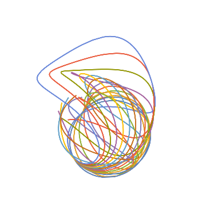 |
Animate the evolution of the curve:
| In[11]:= | ![Animate[ResourceFunction[
"CurvatureTorsionPlot3D"][{1, 1/12 n Sin[t]}, {t, 0, 4 \[Pi]}, Axes -> None, Boxed -> False, ViewPoint -> {1, 1, 2}], {{n, 5}, 1, 12}]](https://www.wolframcloud.com/obj/resourcesystem/images/30b/30b9ee64-cce4-4218-ac05-21db0809f21b/4f824dbe70392ea6.png) |
| Out[11]= | 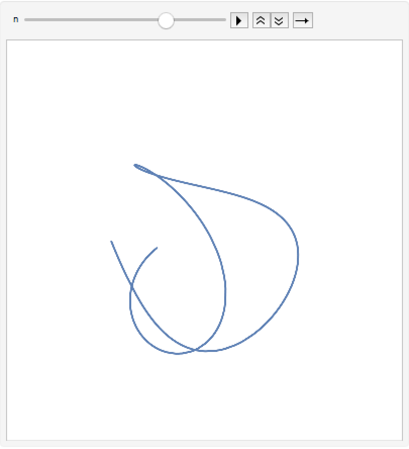 |
Apply a color function:
| In[12]:= |
| Out[12]= | 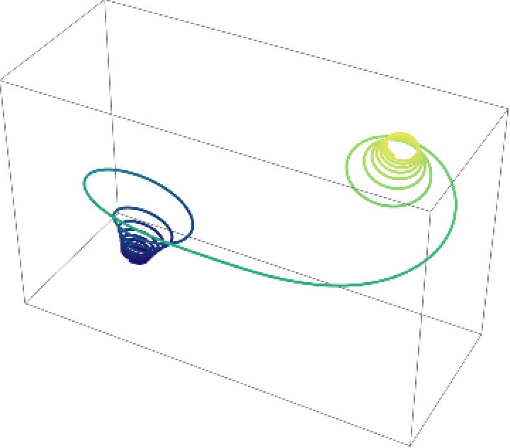 |
Get a curve with prescribed curvature (intrinsic curvature):
| In[13]:= | ![intrinsic[f_, a_, {c_, d_, e_}, {min_, max_}][t_] := Module[{x, y, \[Theta], s, eqic, sol}, eqic = {Derivative[1][x][s] == Cos[\[Theta][s]], Derivative[1][y][s] == Sin[\[Theta][s]], Derivative[1][\[Theta]][s] == f[s], x[a] == c, y[a] == d, \[Theta][a] == e}; sol = NDSolve[eqic, {x, y, \[Theta]}, {s, min, max}]; {x[t], y[t]} /. sol[[1]]];](https://www.wolframcloud.com/obj/resourcesystem/images/30b/30b9ee64-cce4-4218-ac05-21db0809f21b/009c9c102942285f.png) |
Plot a surface of revolution:
| In[14]:= | ![Module[{rad = 1, int = intrinsic[-Sin[#] & , 0, {0, 0, 0}, {-10, 10}][v]}, Show[ParametricPlot3D[
Evaluate[{Cos[u] (rad + int[[1]]), Sin[u] (rad + int[[1]]), int[[2]]}], {u, 0, 2 \[Pi]}, {v, -10, 10}, Mesh -> False, PlotStyle -> Opacity[.5], MaxRecursion -> 3]]]](https://www.wolframcloud.com/obj/resourcesystem/images/30b/30b9ee64-cce4-4218-ac05-21db0809f21b/30349fafd086819e.png) |
| Out[14]= | 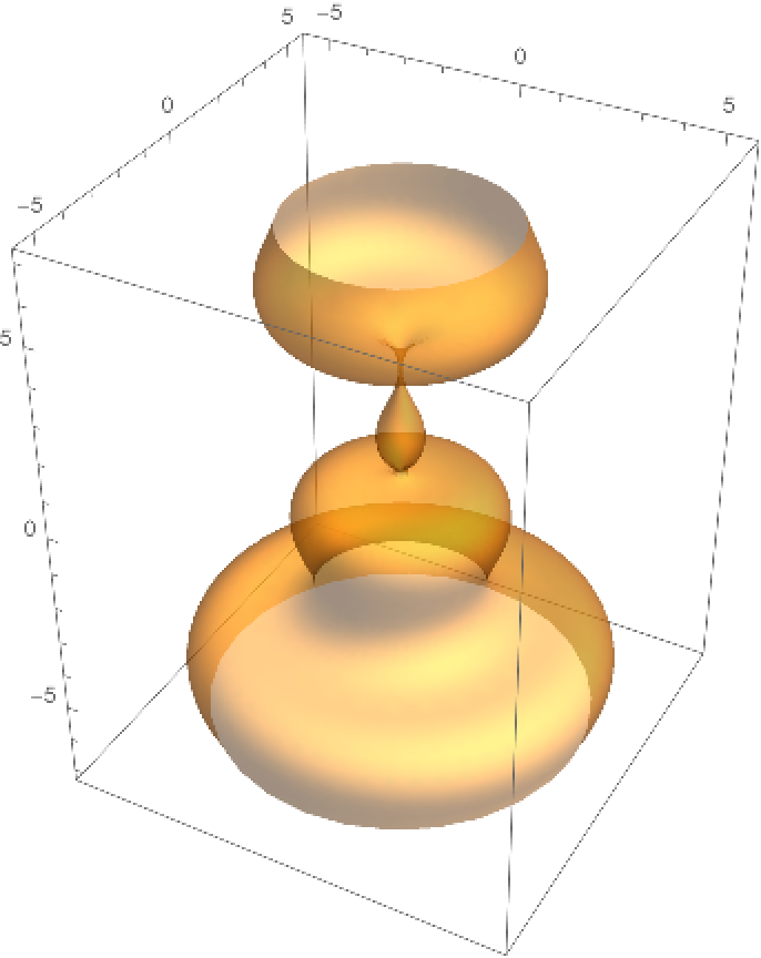 |
Another way to generate a surface with from a curve with intrinsic curvature is by using GeneralizedHelicoid:
| In[15]:= |
| In[16]:= | ![With[{heli = ResourceFunction[
ResourceObject[<|"Name" -> "GeneralizedHelicoid", "ShortName" -> "GeneralizedHelicoid", "UUID" -> "c02813fc-650a-487a-8440-770ef3bbb5db", "ResourceType" -> "Function", "Version" -> "1.0.0", "Description" -> "Compute the generalized helicoid of a curve",
"RepositoryLocation" -> URL[
"https://www.wolframcloud.com/objects/resourcesystem/api/1.0"], "SymbolName" -> "FunctionRepository`$b5251ee2a1154483950ff86636e4c3c2`GeneralizedHelicoid", "FunctionLocation" -> CloudObject[
"https://www.wolframcloud.com/obj/8b8ae647-25d6-4595-903c-37ec6d3616a2"]|>, ResourceSystemBase -> Automatic]][f[v], 0.2, u]}, Show[ParametricPlot3D[heli, {u, 0, 3 \[Pi]/2}, {v, -5, 5}, PlotPoints -> {30, 60}, Mesh -> False, PlotStyle -> Opacity[.5],
MaxRecursion -> 3], ParametricPlot3D[heli /. u -> 0, {v, -5, 5}, Mesh -> False, PlotStyle -> {Opacity[.5], Red}, MaxRecursion -> 3]]
]](https://www.wolframcloud.com/obj/resourcesystem/images/30b/30b9ee64-cce4-4218-ac05-21db0809f21b/46cc174509604032.png) |
| Out[16]= | 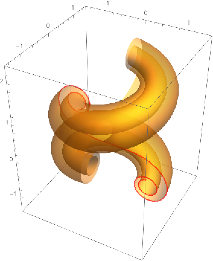 |
This work is licensed under a Creative Commons Attribution 4.0 International License