Basic Examples (2) 

Cube a square matrix:

In[1]:=

Out[1]=

Check the result:

In[2]:=

Out[2]=

Invert a matrix:

In[3]:=

Out[3]=

Check the result:

In[4]:=

Out[4]=

Scope (9) 

Arbitrary differentiable functions of a matrix can be computed provided that the function is well behaved on the matrix eigenvalues:

In[5]:=

Out[5]=

In[6]:=

Out[6]=

Check that the answer is correct:

In[7]:=

Out[7]=

Compute a 10-th power of matrix:

In[8]:=

Out[8]=

In[9]:=

Out[9]=

Check that the computation is correct:

In[10]:=

Out[10]=

A defective matrix:

In[11]:=

Compute its logarithm:

In[12]:=

Out[12]=

Check that computation is correct:

In[13]:=

Out[13]=

This matrix is not diagonalizable:

In[14]:=

Out[14]=

A 2 dimensional matrix:

In[15]:=

Out[15]=

Compute a composition where the second function inverts the first:

In[16]:=

Out[16]=

A matrix function of small matrix can yield a long result:

In[17]:=

Out[17]=

For a multivalued function (for example, fractional power, inverse trigonometric, etc) a single matrix is returned:

In[18]:=

Out[18]=

A check:

In[19]:=

Out[19]=

ComputeMatrixFunction is implemented to handle defective (nondiagonalizable) matrices:

In[20]:=

Out[20]=

The matrix is defective:

In[21]:=

Out[21]=

So the minimal polynomial of this matrix has a factor of nontrivial multiplicity:

In[22]:=

Out[22]=

The minimal polynomial is a polynomial of lowest degree that annihilates the matrix:

In[23]:=

Out[23]=

Compute the exponential of this matrix:

In[24]:=

Out[24]=

Check the size:

In[25]:=

Out[25]=

Symbolic matrices can be input as well:

In[26]:=

Out[26]=

The minimal polynomial has roots with multiplicity greater that one, i.e. the matrix is defective:

In[27]:=

Out[27]=

Since minimal polynomial was already computed, we can help ComputeMatrixFunction by providing a computed matrix polynomial:

In[28]:=

Out[28]=

Compute minimal polynomial for the matrix input*t:

In[29]:=

Out[29]=

Check expOfMatrix using the property 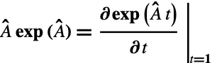of the exponential function to confirm the identity:

In[30]:=

Out[30]=

ComputeMatrixFunction will not work with sparse arrays/structures. Nevertheless, it can deal with larger matrices than MatrixFunction:

In[31]:=

The matrix is non-diagonalizable:

In[32]:=

Out[32]=

Inverse trigonometric functions of a matrix are multi-valued; ComputeMatrixFunction returns only one of them:

In[33]:=

Out[33]=

Verify the huge symbolic result numerically by computing the Sin function:

In[34]:=

Out[34]=

Options (21) 

MinimalPolynomial (4) 

By default the minimal polynomial of matrix is computed using the primitive algorithm described in MatrixMinimalPolynomial; one can instead have the minimal polynomial computed externally.

Give a matrix:

In[35]:=

Out[35]=

The computed minimal polynomial should be provided as a pure function:

In[36]:=

Out[36]=

We can use it inside ComputeMatrixFunction:

In[37]:=

Out[37]=

MatrixFunction returns the same result faster:

In[38]:=

Out[38]=

FunctionDomain (5) 

An input matrix:

In[39]:=

Out[39]=

Compute the matrix exponential in the (default) complex domain:

In[40]:=

Out[40]=

After numerical evaluation we see that negligible imaginary parts are present:

In[41]:=

Out[41]=

Compute the same function in the real domain:

In[42]:=

Out[42]=

Numerical evaluation now shows no imaginary numeric fuzz:

In[43]:=

Out[43]=

OutputSpectralBasis (12) 

The spectral basis1 can be used to compute matrix functions. We illustrate this below, using it to replicate the computation of ComputeMatrixFunction.

Input a matrix:

In[44]:=

Out[44]=

One can compute a given function of matrix along with the generalized spectral basis using option "OutputSpectralBasis"→True:

In[45]:=

Out[45]=

The generalized spectral basis1 is presented as a list of the form {r,plist} where r is a root of the minimal polynomial and plist is a list of polynomials with length equal to the root multiplicity:

In[46]:=

Out[46]=

Compute the minimal polynomial:

In[47]:=

Out[47]=

We see that root -1 has multiplicity 2 so the spectral basis for this root contains two polynomials:

In[48]:=

Out[48]=

Once the spectral basis is known one can compute the matrix function in the following way. For an eigenvalue of multiplicity n we compute derivatives zero through n-1. Since maximal root multiplicity is 2, the zeroth and first derivatives suffice to handle all eigenvalues:

In[49]:=

Out[50]=

Now compute the following sum:

In[51]:=

Out[51]=

First compute the diagonal part of matrix:

In[52]:=

Out[52]=

Then the off-diagonal part:

In[53]:=

Out[53]=

Compute matrix powers up the degree of answerCommutativeVar (7):

In[54]:=

Out[54]=

After replacing formal variable x by the matrix (and similar for powers) we obtain the final answer:

In[55]:=

Out[55]=

Check that it coincides with previously computed exponent of matrix:

In[56]:=

Out[56]=

The manually computed matrix function is considerably simpler due to manual simplification of the generalized spectral basis polynomials. Moreover, other functions of the same matrix can be computed using the same generalized spectral basis, so one can compute multiple function computation of the same matrix.

Properties and Relations (2) 

Define a matrix:

In[57]:=

An arbitrary polynomial p for which p(A)=0, for example the characteristic polynomial, can be provided as a pure function:

In[58]:=

Out[58]=

Also compute minimal polynomial:

In[59]:=

Out[59]=

Compute the product of the characteristic and minimal polynomials:

In[60]:=

Out[60]=

Computation time increases with the degree of provided polynomial, since higher matrix powers get computed:

In[61]:=

Out[61]=

In[62]:=

Out[62]=

ComputeMatrixFunction is similar to the built-in MatrixFunction but often yields a less complicated result than in a fraction of time:

In[63]:=

Out[63]=

Compare with MatrixFunction:

In[64]:=

Out[64]=

Numerical comparison of both results up to 100 digits takes over 10 minutes, so instead compare an arbitrary element (1,3):

In[65]:=

Out[65]=

Possible Issues (2) 

A noninvertible matrix:

In[66]:=

If the given function is not defined at matrix eigenvalues then the computation will fail:

In[67]:=

Out[67]=

We can determine a problem by inserting formal function f:

In[68]:=

Out[68]=

The algorithm tries to evaluate function and it's derivatives at points 0 and 2:

In[69]:=

Out[69]=

It is clear that the attempt to compute reciprocals 1/eigval at 0 produced the error.

ComputeMatrixFunction, like MatrixFunction, does not work with non-differentiable functions such as Abs:

In[70]:=

Out[70]=

The result is meaningless because Abs does not have a first or second derivative.