Wolfram Function Repository
Instant-use add-on functions for the Wolfram Language
Function Repository Resource:
Give a color function a periodic perturbation
ResourceFunction["ColorFunctionRipple"][cf] introduces periodic perturbations to the color function cf. |
| "Profile" | "Waves" | the shape of the perturbation |
| "Frequency" | 1 | how often the perturbations occur |
| "Waves" | |
| "Layers" | |
| "Crenels" | |
| "Gullets" | |
| "Hills" | |
| "Troughs" |
Show a rippled gradient:
| In[1]:= |
| Out[1]= |
Modify a color gradient represented as a pure function:
| In[2]:= |
| Out[2]= |
Modify a color gradient from the WFR:
| In[3]:= | ![LinearGradientImage[
ResourceFunction[
"ColorFunctionRipple"][(ResourceFunction["ViridisColor"][{"Plasma", "Reverse"}, #]) &], {600, 40}]](https://www.wolframcloud.com/obj/resourcesystem/images/87d/87d63d1b-a9bf-46b2-a9aa-ec04966044b0/5fc226216970cd44.png) |
| Out[3]= |
Select a profile shape that best suits your needs:
| In[4]:= | ![Column[Table[
Graphics[{Raster[{Range[500]/500}, ColorFunction -> ResourceFunction["ColorFunctionRipple"]["StarryNightColors", "Profile" -> p]], Text[Style[p, 14], {480, .5}, {1, 0}]}, AspectRatio -> .08, PlotRangePadding -> .1, ImageSize -> 600], {p, {"Waves", "Crenels", "Hills", "Layers", "Troughs", "Gullets"}}], Spacings -> 0]](https://www.wolframcloud.com/obj/resourcesystem/images/87d/87d63d1b-a9bf-46b2-a9aa-ec04966044b0/28fa2dfb3c0e390e.png) |
| Out[4]= | 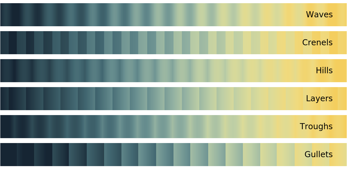 |
Increase or decrease the number of ripples along the color function:
| In[5]:= | ![Column[Table[
Graphics[{Raster[{Range[500]/500}, ColorFunction -> ResourceFunction["ColorFunctionRipple"]["CherryTones", "Frequency" -> p]], Text[Style[ToString[p], 14], {480, .5}, {1, 0}]}, AspectRatio -> .08, PlotRangePadding -> .1, ImageSize -> 600], {p, {.5, 1, 2, 4}}], Spacings -> 0]](https://www.wolframcloud.com/obj/resourcesystem/images/87d/87d63d1b-a9bf-46b2-a9aa-ec04966044b0/307e2e5bea6b7828.png) |
| Out[5]= | 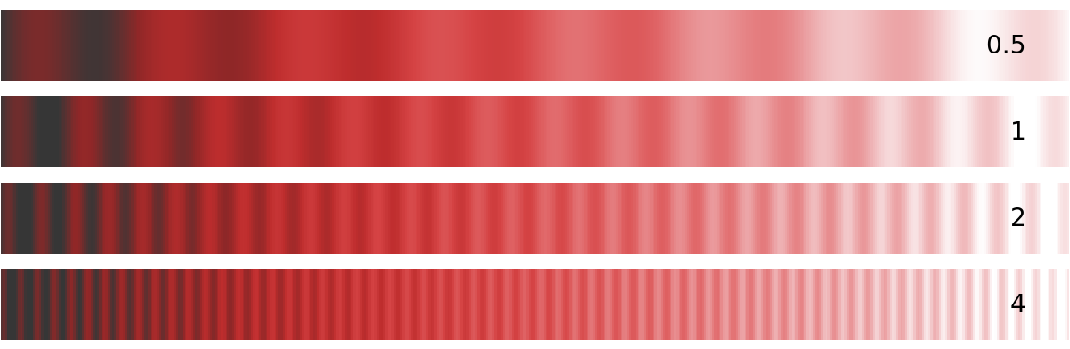 |
Style a plot:
| In[6]:= | ![cf = Blend[{{0, Darker[Blue]}, {1, White}}, #] &;
Plot[Sin[x], {x, 0, 2 \[Pi]}, PlotStyle -> AbsoluteThickness[10], ColorFunction -> ResourceFunction["ColorFunctionRipple"][cf, "Profile" -> "Crenels"],
AspectRatio -> .5, ImageSize -> 500]](https://www.wolframcloud.com/obj/resourcesystem/images/87d/87d63d1b-a9bf-46b2-a9aa-ec04966044b0/6c99605930f28ddb.png) |
| Out[7]= | 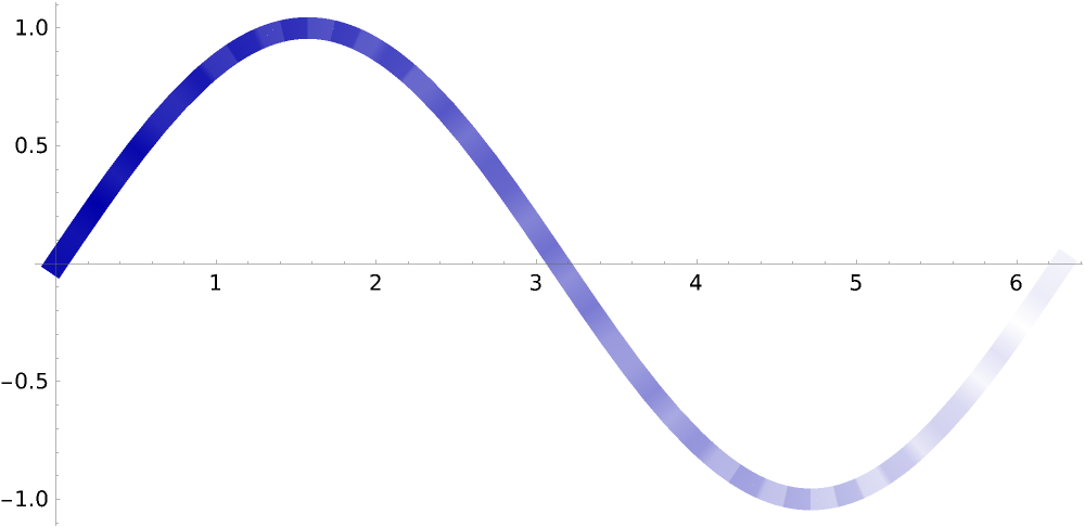 |
Style a 3D shape:
| In[8]:= | ![ContourPlot3D[x^2 + y^2 + z^2, {x, -2, 2}, {y, -2, 2}, {z, -2, 2}, PlotPoints -> 100, MeshStyle -> None, Boxed -> False, ColorFunction -> ResourceFunction["ColorFunctionRipple"][Hue[#2, 2 #2, 2 #2] &], Axes -> None]](https://www.wolframcloud.com/obj/resourcesystem/images/87d/87d63d1b-a9bf-46b2-a9aa-ec04966044b0/313bd241c5a4254e.png) |
| Out[23]= | 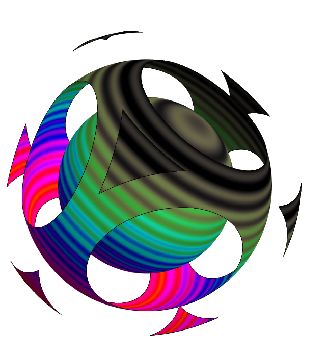 |
Alter the surface colors of a relief plot:
| In[24]:= | ![ReliefPlot[
Table[x + Sin[3 x + y^2], {x, -4, 4, 0.05}, {y, -4, 4, 0.05}], ColorFunction -> ResourceFunction["ColorFunctionRipple"]["SunsetColors", "Frequency" -> .5]]](https://www.wolframcloud.com/obj/resourcesystem/images/87d/87d63d1b-a9bf-46b2-a9aa-ec04966044b0/53c0fc6789caee35.png) |
| Out[24]= | 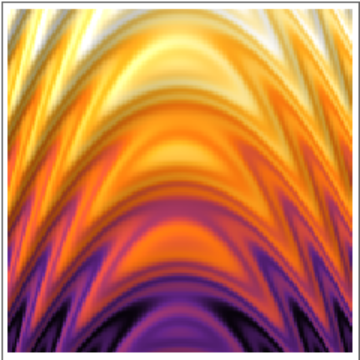 |
ColorFunctionRipple currently does not support pure functions with named arguments:
| In[25]:= | ![LinearGradientImage[
ResourceFunction["ColorFunctionRipple"][
Function[t, ColorData["M10DefaultDensityGradient"][t]]], {600, 40}]](https://www.wolframcloud.com/obj/resourcesystem/images/87d/87d63d1b-a9bf-46b2-a9aa-ec04966044b0/3f9e10728ce472d3.png) |
| Out[25]= |
Use the gradient name directly instead:
| In[26]:= |
| Out[26]= |
Create interesting visual effects:
| In[27]:= | ![ParametricPlot3D[
Evaluate[
RotationTransform[
2 \[Pi] v, {0, 0, 1}][.5^
v {Cos[2 \[Pi] u], 0, Sin[2 \[Pi] u]}] + .5^
v {Cos[2 \[Pi] v], Sin[2 \[Pi] v], -2.4}],
{u, 0, 1}, {v, 0, 8},
PlotRange -> All, MaxRecursion -> 4, Mesh -> None, Boxed -> False, Axes -> False, PlotPoints -> 100,
ColorFunction -> ResourceFunction["ColorFunctionRipple"][ColorData["Pastel"][#4] &, "Profile" -> "Hills"]]](https://www.wolframcloud.com/obj/resourcesystem/images/87d/87d63d1b-a9bf-46b2-a9aa-ec04966044b0/598bfde4a2a2a325.png) |
| Out[27]= | 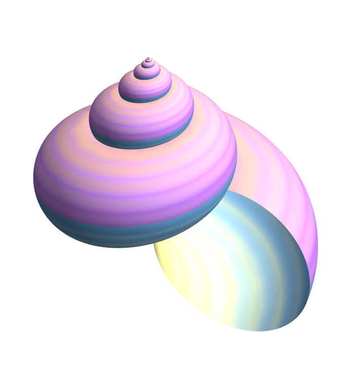 |
This work is licensed under a Creative Commons Attribution 4.0 International License