Wolfram Function Repository
Instant-use add-on functions for the Wolfram Language
Function Repository Resource:
Create a diverging color map with a neutral central color
ResourceFunction["DivergentColorFunction"][col1, col2] returns a diverging color map that interpolates between col1 and col2, with a neutral, unsaturated color in the center of the input range. | |
ResourceFunction["DivergentColorFunction"]["CoolToWarm"] returns the color map demonstrated in the paper "Diverging Color Maps for Scientific Visualization" by Kenneth Moreland. | |
Choose two colors and create a color function from them:
| In[1]:= |
| Out[1]= |
| In[2]:= |
| Out[2]= |
| In[3]:= |
| Out[3]= | 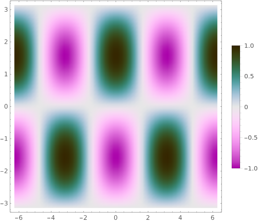 |
Create a color function using a built-in color scheme:
| In[4]:= | ![DensityPlot[Cos[x] Sin[y], {x, -2 \[Pi], 2 \[Pi]}, {y, -\[Pi], \[Pi]},
ColorFunction -> ResourceFunction["DivergentColorFunction"]["RoseColors"], PlotLegends -> Automatic, PlotPoints -> 50]](https://www.wolframcloud.com/obj/resourcesystem/images/9ea/9ea81b32-459d-48f1-86b3-955bfd372116/072e9d2473a6f328.png) |
| Out[4]= | 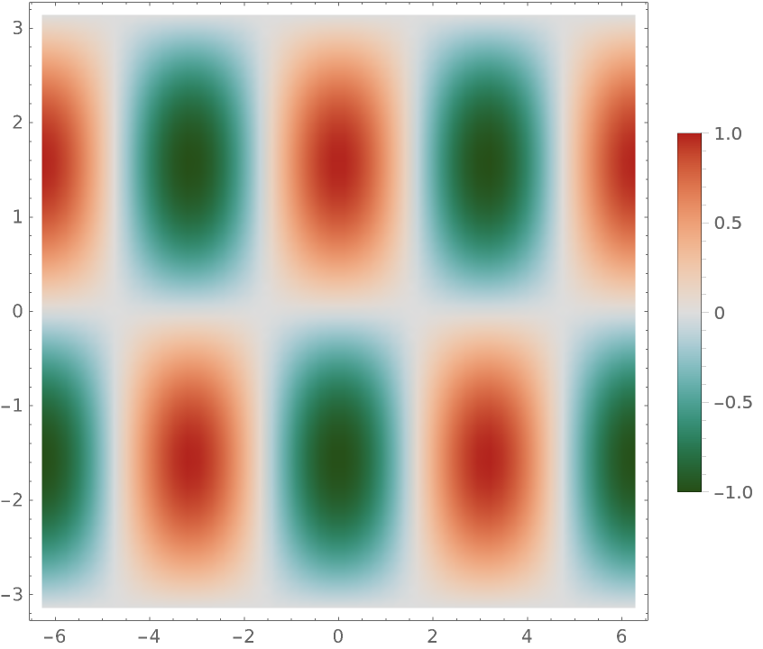 |
Compare this with the same plot using the unmodified scheme:
| In[5]:= |
| Out[5]= | 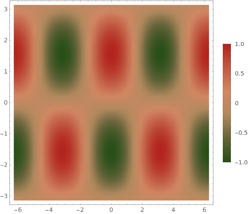 |
Create a plotting function to visualize color maps:
| In[6]:= | ![showcolorfunction[color_] := With[{opts = {PlotRange -> All, ColorFunction -> color, PlotPoints -> 40, PlotRangePadding -> None, ImageSize -> 200}}, Column[{DensityPlot[
Cos[x] Sin[y], {x, -2 \[Pi], 2 \[Pi]}, {y, -\[Pi], \[Pi]}, FrameTicks -> None, AspectRatio -> 1/4, opts], DensityPlot[
10 Cos[x^2] Exp[y], {x, -2 \[Pi], 2 \[Pi]}, {y, -\[Pi], 0}, FrameTicks -> None, AspectRatio -> 1/2, opts], DensityPlot[x, {x, -1, 1}, {y, 0, 1}, FrameTicks -> {{None, None}, {Automatic, None}}, AspectRatio -> 1/10, opts]}, Center, 0]];](https://www.wolframcloud.com/obj/resourcesystem/images/9ea/9ea81b32-459d-48f1-86b3-955bfd372116/004d29d4071b6a2f.png) |
Now recreate the example color functions from Kenneth Moreland’s "Diverging Color Maps for Scientific Visualization":
| In[7]:= | ![showcolorfunction /@ ResourceFunction[
"DivergentColorFunction"] @@@ {{{0.23, 0.299, 0.754}, {0.706, 0.016,
0.150}}, {{0.436, 0.308, 0.631}, {0.759, 0.334, 0.046}}, {{0.085, 0.532, 0.201}, {0.436, 0.308, 0.631}}, {{0.217,
0.525, 0.910}, {0.677, 0.492, 0.093}}, {{0.085, 0.532, 0.201}, {0.758, 0.214, 0.233}}}](https://www.wolframcloud.com/obj/resourcesystem/images/9ea/9ea81b32-459d-48f1-86b3-955bfd372116/6c18cfbe2f89a3b8.png) |
| Out[7]= | 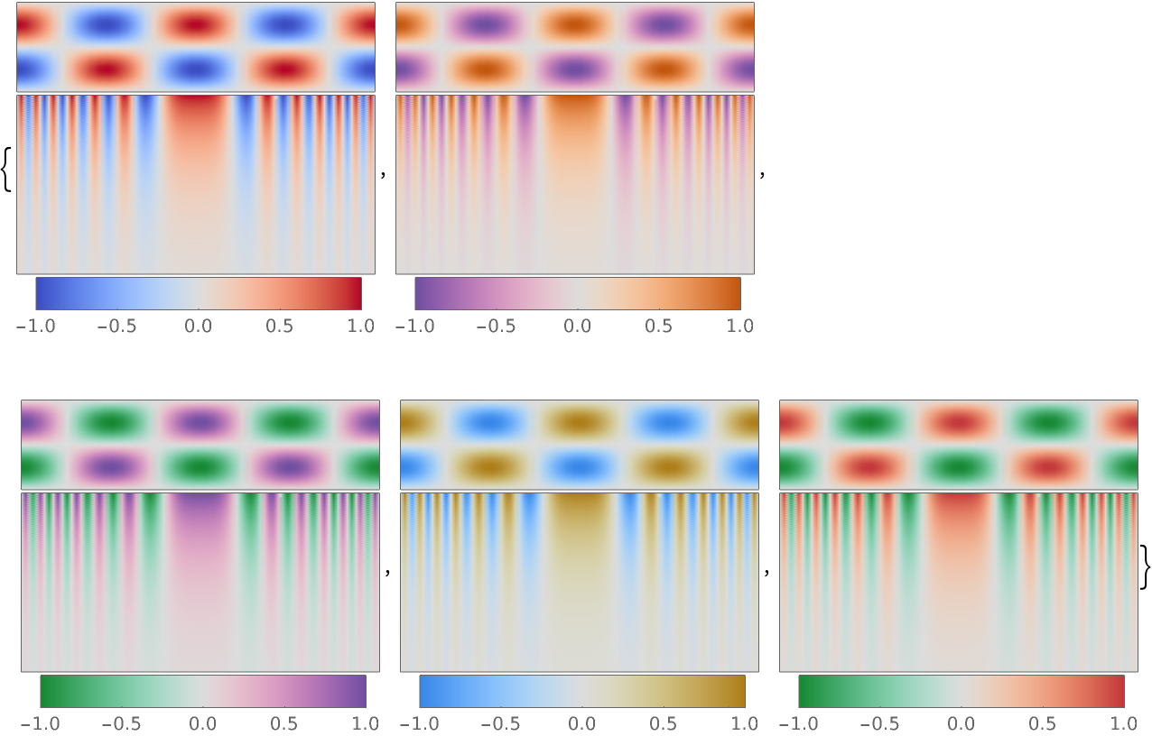 |
Wolfram Language 11.3 (March 2018) or above
This work is licensed under a Creative Commons Attribution 4.0 International License