Function Repository Resource:

ClickPoincarePlot2D

Create an interactive view of Poincaré sections of a two-degree-of-freedom Hamiltonian system

Contributed by: E. Chan-López, Héctor Argote Morales, Wojciech Szumiński & Víctor Castellanos

ResourceFunction["ClickPoincarePlot2D"][odes,h,energy,time,timemax,cross,recover]

gives the Poincaré sections corresponding to the differential equations represented by odes, the Hamiltonian h, the energy level energy, the time variable time, the maximum time of evolution timemax, the intersection cross and the section recover, with initial conditions determined by clicking within an interactive panel.

ResourceFunction["ClickPoincarePlot2D"][odes,h,energy,time,timemax,cross,recover,name]

include name as a label.

Details and Options

Formally, in classical mechanics, the Hamiltonian is a mathematical function that ResourceFunction["ClickPoincarePlot2D"] describes the total energy (kinetic and potential energies) of a physical system, considering all interactions between its constituents. It is denoted by H and is defined in terms of the coordinates and generalized momenta of the system.

The temporal evolution of the Hamiltonian system is governed by Hamilton's equations. These equations arise from the Hamiltonian function using the Poisson Bracket.

Formally, a Hamiltonian system refers to a physical system described within the framework of Hamiltonian mechanics. In this approach, the system is characterized by its phase space, which is an abstract space where each point represents a set of generalized coordinates and their corresponding conjugate momenta.

The odes must be a list of ordinary differential equations, specifically a Hamiltonian system.

The h must be a Hamiltonian function.

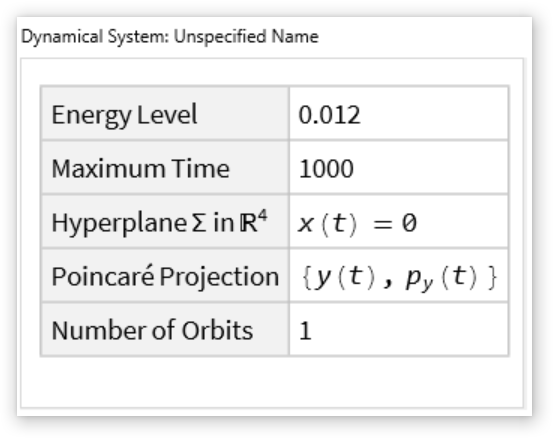
The energy must be a numeric expression. The variable energy represents the energy level chosen when painting a Poincaré section. It is a parameter that determines the specific energy value at which the section is taken. By selecting different values of energy, one can explore different energy regimes and capture distinct features of the dynamical system on the Poincaré section.

The cross should be a time-dependent variable. It can also be an equation, where its left-hand side is a time-dependent variable and its right-hand side is a constant. The argument cross represents the crossing plane of the solutions.

The recover must be a list of two time-dependent variables. This list indicates the plane where the points of each section will be collected.

ResourceFunction["ClickPoincarePlot2D"] collects the data of the initial value together with the data of the associated orbit, this depending on the points that the user chooses in the clickable panel, also drawing the respective section.

ResourceFunction["ClickPoincarePlot2D"] takes the same options as ListPlot.

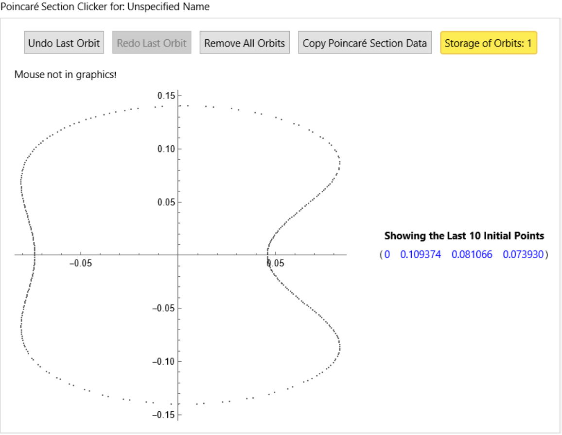
ResourceFunction["ClickPoincarePlot2D"] name is an optional argument (default: "Unspecified Name") used to label the Poincaré sections in the interface. If no name is provided, the default label "Unspecified Name" will be used.

Examples

Basic Examples (2)

Generate a Poincaré section of the following system:

In[1]:=

$H[{x_, px_, y_, py_}] := 1/2 (px^2 + py^2 + x^2 + y^2) + 2 x^2*y; eqns = {x'[t] == px[t], px'[t] == -x[t] (1 + 2 y[t]), y'[t] == py[t], py'[t] == -x[t]^2 - y[t] };$

In[2]:=

Out[2]=

Obtain the orbits and initial points by clicking the button labeled Copy Poincaré Section Data. Initially, a Dataset is displayed as a summary with ClickToCopy enabled, allowing you to copy the data. The orbit data and initial points are provided as an iconized Association with the keys "Orbits" and "Initial Points":

Applications (8)

Chaotic Regime in the Hénon-Heiles Equation (1)

Generate Poincaré sections of the Hénon-Heiles Equation under chaotic regime:

In[3]:=

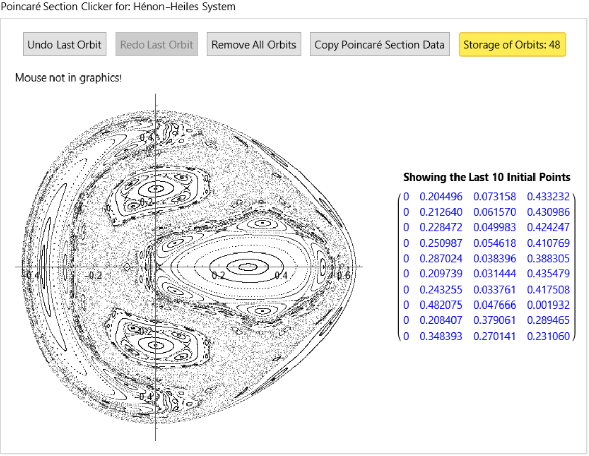
$H1[{x_, px_, y_, py_}] := 1/2 (px^2 + py^2 + x^2 + y^2) + x^2*y - 1/3 y^3; hamEqns1 = {x'[t] == px[t], px'[t] == -(x[t] + 2 x[t]* y[t]), y'[t] == py[t], py'[t] == -(y[t] + x[t]^2 - y[t]^2) }; name = "Hénon-Heiles System";$

In[4]:=

Out[4]=

Dynamics of a Relativistic Hénon-Heiles System (1)

Generate Poincaré sections of the relativistic Hénon-Heiles system:

In[5]:=

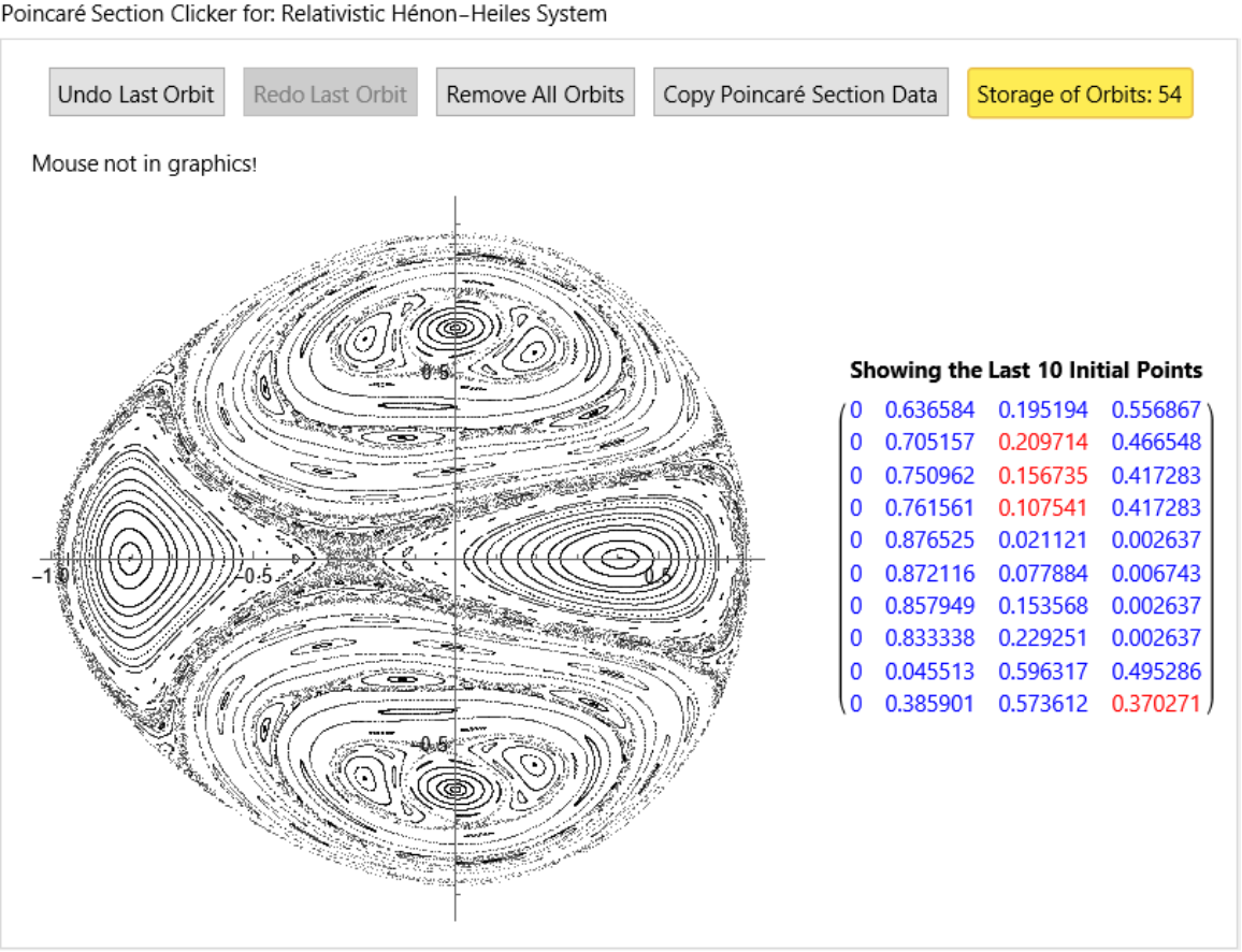
$eMin = 1; H2[{q1_, p1_, q2_, p2_}] := Sqrt[1 + p1^2 + p2^2] + 1/2 (q1^2 + q2^2) + \[Alpha]*q1^2 q2 + 1/3 \[Beta]*q2^3 /. {\[Alpha] -> 1/2, \[Beta] -> 1/2}; hamEqns2 = {q1'[t] == p1[t]/Sqrt[1 + p1[t]^2 + p2[t]^2], p1'[t] == -q1[t] (1 + q2[t]), q2'[t] == p2[t]/Sqrt[1 + p1[t]^2 + p2[t]^2], p2'[t] == 1/2 (-q1[t]^2 - q2[t] (2 + q2[t])) }; name = "Relativistic Hénon-Heiles System";$

In[6]:=

Out[6]=

Dynamics of a Rydberg Atom in a Dielectric Cavity (1)

Generate Poincaré sections for a system of a Rydberg atom in a dielectric cavity under the chaotic regime:

In[7]:=

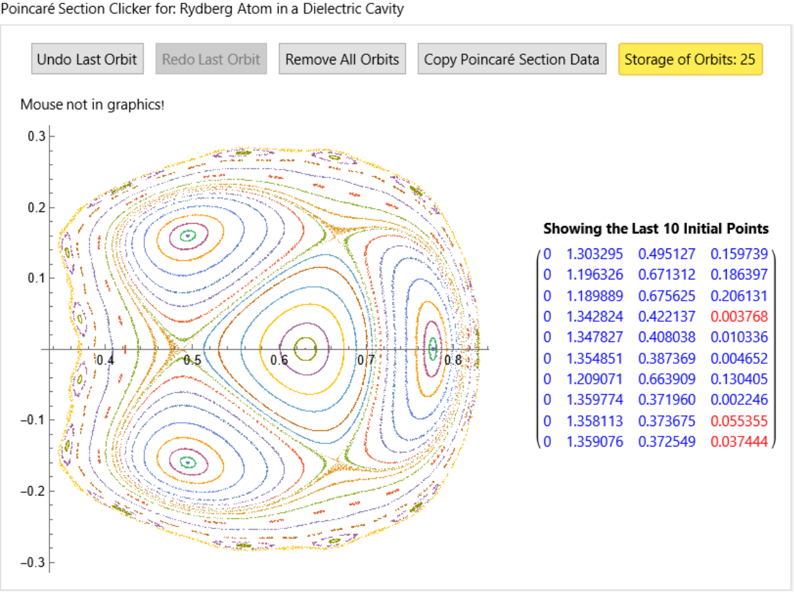
$a = (\[Epsilon]2 - \[Epsilon]1)/(\[Epsilon]2 + \[Epsilon]1); b = (\[Epsilon]2 - \[Epsilon]3)/(\[Epsilon]2 + \[Epsilon]3); c = ((\[Epsilon]2 - \[Epsilon]1) (\[Epsilon]2 - \[Epsilon]3))/((\[Epsilon]2 + \[Epsilon]1) (\[Epsilon]2 + \[Epsilon]3)); \[CurlyEpsilon]0 = -21/40;$

In[8]:=

$H3[{u_, pu_, v_, pv_}] := ((pu)^2 + (pv)^2)/ 2 - (u^2 + v^2) \[CurlyEpsilon] - Z/\[Epsilon]2 (a (u^2 + v^2))/Sqrt[ u^2 v^2 + (2 \[Zeta] + ((u^2 - v^2)/2))^2] - Z/\[Epsilon]2 (b (u^2 + v^2))/Sqrt[ u^2 v^2 + (2 - 2 \[Zeta] - ((u^2 - v^2)/2))^2] - Z/\[Epsilon]2 (c (u^2 + v^2))/Sqrt[ u^2 v^2 + (2 + (u^2 - v^2)/2)^2] - Z/\[Epsilon]2 (c (u^2 + v^2))/Sqrt[ u^2 v^2 + (2 - (u^2 - v^2)/2)^2] + 1/(4 \[Epsilon]2) ((a (u^2 + v^2))/(\[Zeta] - (u^2 - v^2)/2) + ( b (u^2 + v^2))/(1 - \[Zeta] - (u^2 - v^2)/2)) /. {\[Zeta] -> 8/10, Z -> 2, \[Epsilon]1 -> 10, \[Epsilon]2 -> 4, \[Epsilon]3 -> 3, \[CurlyEpsilon] -> \[CurlyEpsilon]0};$

In[9]:=

$hamEqns3 = { u'[t] == pu[t], pu'[t] == u[ t] (2 \[CurlyEpsilon] - (8 (-(4/5) + u[t]^2 - 3 v[t]^2))/( 35 (u[t]^4 + 2 u[t]^2 (-(4/5) + v[t]^2) + (4/5 + v[t]^2)^2)^( 3/2)) - (96 (16/5 + u[t]^2 - 3 v[t]^2))/( 35 (u[t]^4 + (-(16/5) + v[t]^2)^2 + 2 u[t]^2 (16/5 + v[t]^2))^(3/2)) - ( 24 (4 + u[t]^2 - 3 v[t]^2))/( 49 (u[t]^4 + (-4 + v[t]^2)^2 + 2 u[t]^2 (4 + v[t]^2))^( 3/2)) + (24 (-4 + u[t]^2 - 3 v[t]^2))/( 49 (u[t]^4 + 2 u[t]^2 (-4 + v[t]^2) + (4 + v[t]^2)^2)^( 3/2)) + 1/ 2 (-((1/5 + v[t]^2)/(7 (2/5 - u[t]^2 + v[t]^2)^2)) + ( 3 (4/5 + v[t]^2))/(7 (8/5 - u[t]^2 + v[t]^2)^2))), v'[t] == pv[t], pv'[t] == v[t] (2 \[CurlyEpsilon] + (8 (4/5 - 3 u[t]^2 + v[t]^2))/( 35 (u[t]^4 + 2 u[t]^2 (-(4/5) + v[t]^2) + (4/5 + v[t]^2)^2)^( 3/2)) + (96 (-(16/5) - 3 u[t]^2 + v[t]^2))/( 35 (u[t]^4 + (-(16/5) + v[t]^2)^2 + 2 u[t]^2 (16/5 + v[t]^2))^(3/2)) + ( 24 (-4 - 3 u[t]^2 + v[t]^2))/( 49 (u[t]^4 + (-4 + v[t]^2)^2 + 2 u[t]^2 (4 + v[t]^2))^( 3/2)) - (24 (4 - 3 u[t]^2 + v[t]^2))/( 49 (u[t]^4 + 2 u[t]^2 (-4 + v[t]^2) + (4 + v[t]^2)^2)^( 3/2)) + 1/ 2 (-((1/5 - u[t]^2)/(7 (2/5 - u[t]^2 + v[t]^2)^2)) + ( 3 (4/5 - u[t]^2))/(7 (8/5 - u[t]^2 + v[t]^2)^2))) } /. \[CurlyEpsilon] -> \[CurlyEpsilon]0; name = "Rydberg Atom in a Dielectric Cavity";$

In[10]:=

Out[10]=

Dynamics of a Rydberg Atom Near a Topologically Insulating Surface (1)

Generate Poincaré sections for a system of a Rydberg atom near a topologically insulating surface under the chaotic regime:

In[11]:=

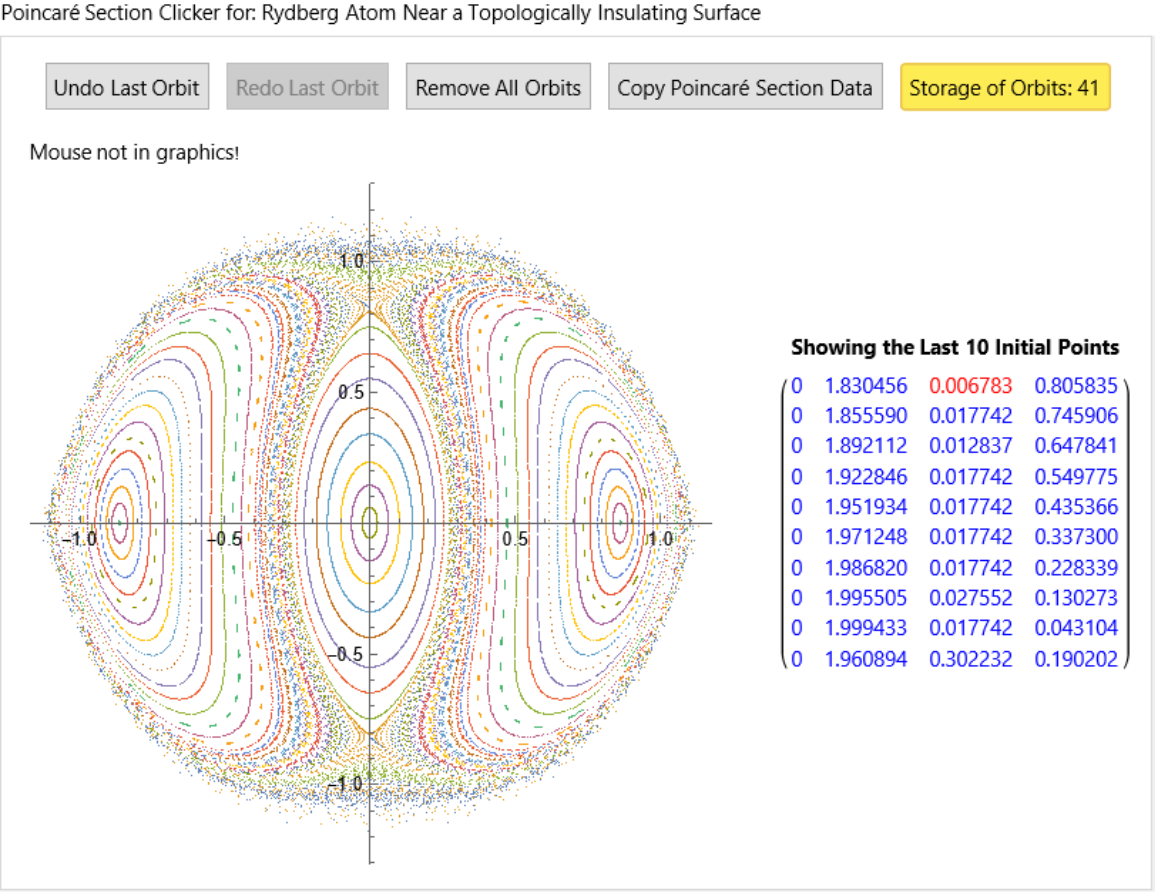
$H4[{u_, pu_, v_, pv_}] := ((pu)^2 + (pv)^2)/ 2 - (u^2 + v^2) \[Epsilon] + (2 \[Alpha] (u^2 + v^2))/(\[Sqrt](4 u^2 v^2 + (u^2 - v^2 + 4)^2)) - (\[Alpha] (u^2 + v^2))/( 2 (u^2 - v^2 + 2)) /. {\[Epsilon] -> -1/2, \[Alpha] -> 3/5} ; hamEqns4 = { u'[t] == pu[t], pu'[t] == 2 u[t] \[Epsilon] + (u[t] \[Alpha])/( 2 + u[t]^2 - v[t]^2) - (u[t] (u[t]^2 + v[t]^2) \[Alpha])/(2 + u[t]^2 - v[t]^2)^2 + (4 u[ t] (u[t]^2 + v[t]^2) (4 + u[t]^2 + v[t]^2) \[Alpha])/(u[ t]^4 + (-4 + v[t]^2)^2 + 2 u[t]^2 (4 + v[t]^2))^( 3/2) - (4 u[ t] \[Alpha])/(\[Sqrt](u[t]^4 + (-4 + v[t]^2)^2 + 2 u[t]^2 (4 + v[t]^2))), v'[t] == pv[t], pv'[t] == 2 v[t] \[Epsilon] + (v[t] \[Alpha])/( 2 + u[t]^2 - v[t]^2) + (v [t] (u[t]^2 + v[t]^2) \[Alpha])/(2 + u[t]^2 - v[t]^2)^2 + (4 v[ t] (u[t]^2 + v[t]^2) (-4 + u[t]^2 + v[t]^2) \[Alpha])/(u[ t]^4 + (-4 + v[t]^2)^2 + 2 u[t]^2 (4 + v[t]^2))^( 3/2) - (4 v[ t] \[Alpha])/(\[Sqrt](u[t]^4 + (-4 + v[t]^2)^2 + 2 u[t]^2 (4 + v[t]^2))) } /. {\[Epsilon] -> -1/2, \[Alpha] -> 3/5} ; name = "Rydberg Atom Near a Topologically Insulating Surface";$

In[12]:=

Out[12]=

Relativistic Anisotropic Harmonic Oscillator (1)

Generate the Poincaré sections of the relativistic anisotropic harmonic oscillator:

In[13]:=

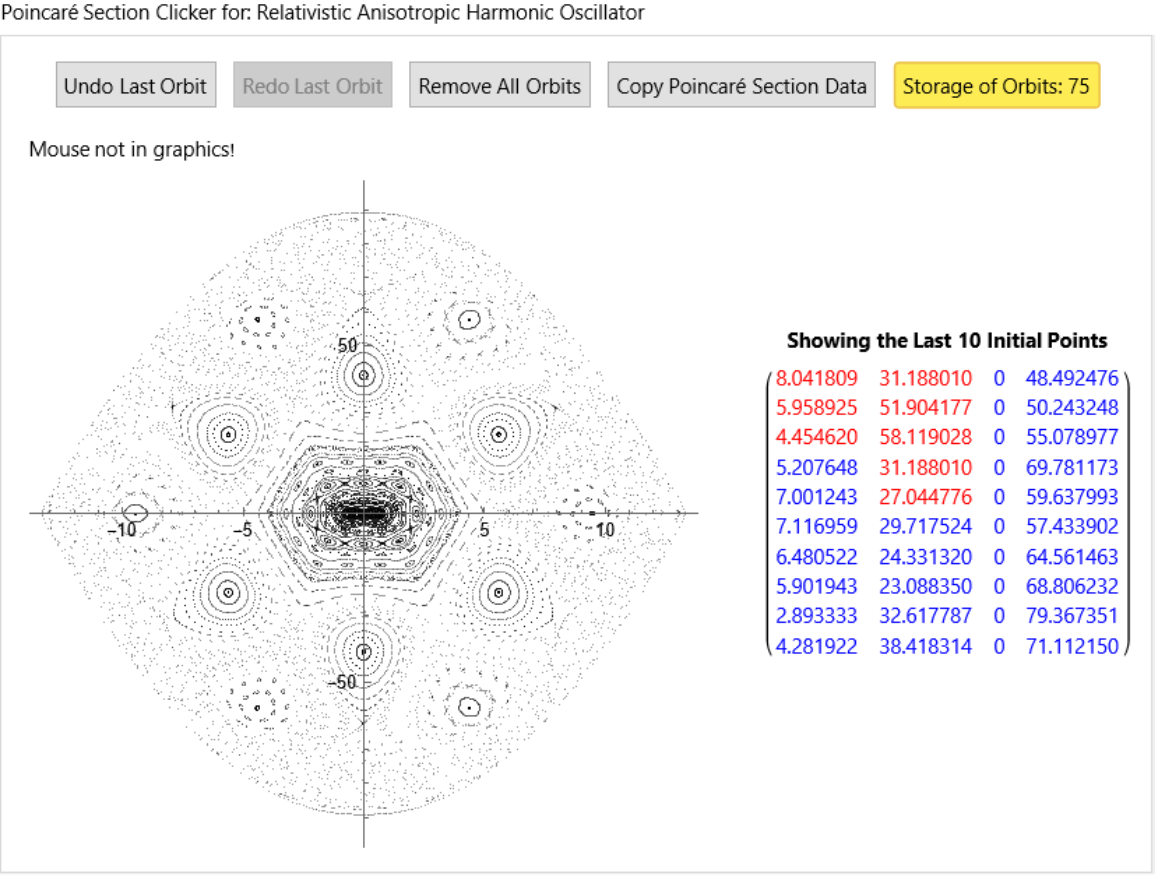
$H5[{x_, px_, y_, py_}] := Sqrt[1 + px^2 + py^2] + x^2/2 + y^2/2 + y^4/80; hamEqns5 = {x'[t] == px[t]/Sqrt[1 + px[t]^2 + py[t]^2], px'[t] == -x[t], y'[t] == py[t]/Sqrt[1 + px[t]^2 + py[t]^2], py'[t] == -y[t] - y[t]^3/20 }; name = "Relativistic Anisotropic Harmonic Oscillator";$

In[14]:=

Out[14]=

Rydberg Hydrogen Atom Near a Metallic Surface (1)

Generate the Poincaré sections for the Rydberg hydrogen atom near a metallic surface:

In[15]:=

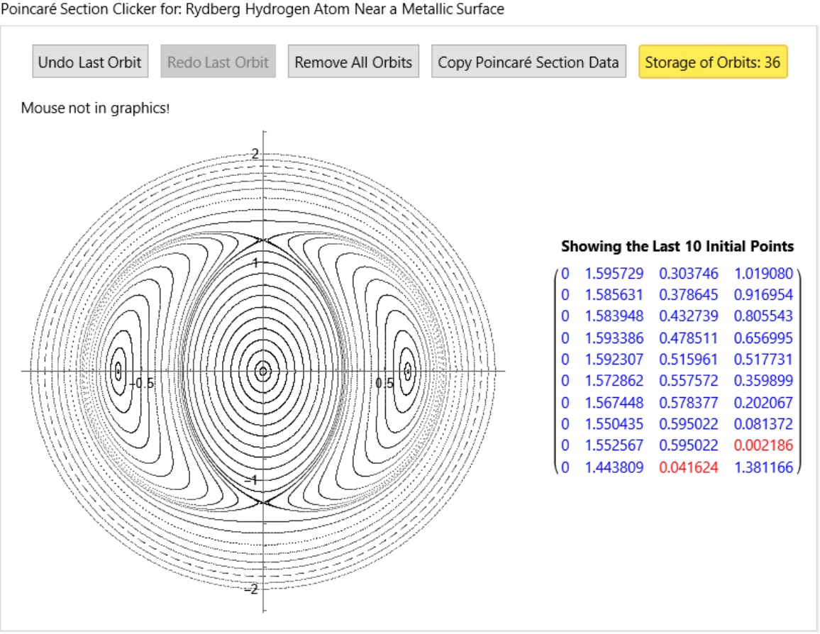
$\[Xi] = -2; H6[{u_, pu_, v_, pv_}] := 1/2 (pu^2 + pv^2) - \[Xi] (u^2 + v^2) - (u^2 + v^2)/( 2 (2 + u^2 - v^2)) + (2 (u^2 + v^2))/Sqrt[ 4 u^2 v^2 + (4 + (u^2 - v^2))^2]; hamEqns6 = {u'[t] == pu[t], pu'[t] == u[t] (2 \[Xi] - (2 (-1 + v[t]^2))/(2 + u[t]^2 - v[t]^2)^2 - ( 16 (4 + u[t]^2 - 3 v[t]^2))/(u[t]^4 + (-4 + v[t]^2)^2 + 2 u[t]^2 (4 + v[t]^2))^(3/2)), v'[t] == pv[t], pv'[t] == v[t] (2 \[Xi] + (2 (1 + u[t]^2))/(2 + u[t]^2 - v[t]^2)^2 - ( 16 (4 + 3 u[t]^2 - v[t]^2))/(u[t]^4 + (-4 + v[t]^2)^2 + 2 u[t]^2 (4 + v[t]^2))^(3/2)) }; name = "Rydberg Hydrogen Atom Near a Metallic Surface";$

In[16]:=

Out[16]=

The Galactic Model of Contopoulos (1)

Generate the Poincaré sections for the Contopoulos model:

In[17]:=

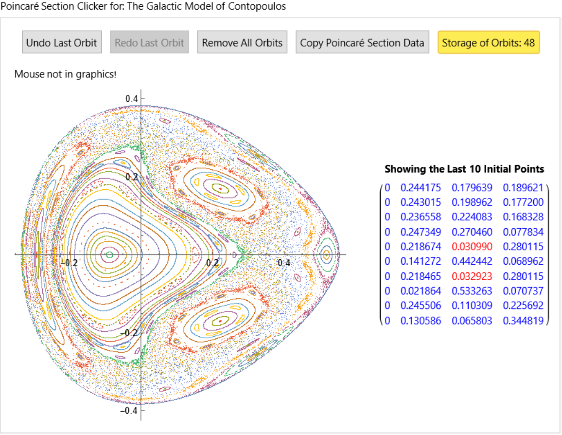
$H7[{x1_, px1_, x2_, px2_}] := px1^2/2 + px2^2/(2 Sqrt[2]) + x2^2/(2 Sqrt[2]) - x2^3/3 + x1^2 (1/2 + x2); hamEqns7 = {x1'[t] == px1[t], px1'[t] == -x1[t] (1 + 2 x2[t]), x2'[t] == px2[t]/Sqrt[2], px2'[t] == -x1[t]^2 - (1/Sqrt[2] - x2[t]) x2[t] }; name = "The Galactic Model of Contopoulos";$

In[18]:=

Out[18]=

The Swing-Spring (1)

Generate the Poincaré sections of the swing-spring:

In[19]:=

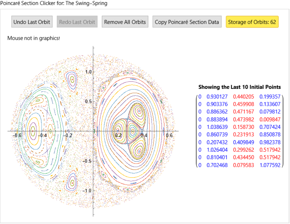
$H8[{x_, px_, z_, pz_}] := 1/2 (px^2 + pz^2) + z + 2 (3/4 - Sqrt[x^2 + (z - 1)^2])^2 - 1/8; hamEqns8 = { x'[t] == px[t], px'[t] == x[t] (-4 + 3/Sqrt[x[t]^2 + (-1 + z[t])^2]), z'[t] == pz[t], pz'[t] == 3 - 3/Sqrt[ x[t]^2 + (-1 + z[t])^2] + (-4 + 3/Sqrt[ x[t]^2 + (-1 + z[t])^2]) z[t] }; name = "The Swing-Spring";$

In[20]:=

Out[20]=

Publisher

Ramón Eduardo Chan López

Requirements

Wolfram Language 13.0 (December 2021) or above

Version History

2.0.0 – 14 March 2025
1.0.1 – 02 October 2023
1.0.0 – 13 July 2023

Source Metadata

Citation:
- Giorgilli, A. (2022). Notes on Hamiltonian Dynamical Systems (Vol. 102). Cambridge University Press. DOI: 10.1017/9781009151122
- Lowenstein, J. H. (2012). Essentials of Hamiltonian dynamics. Cambridge University Press. DOI: 10.1017/CBO9780511793721
- Vieira, R. S., & Michtchenko, T. A. (2018). Relativistic chaos in the anisotropic harmonic oscillator. Chaos, Solitons & Fractals, 117, 276-282. DOI: 10.1016/j.chaos.2018.10.027
- van der Weele, J. P., & de Kleine, E. (1996). The order—chaos—order sequence in the spring pendulum. Physica A: Statistical Mechanics and its Applications, 228(1-4), 245-272. DOI: 10.1016/0378-4371(95)00426-2
- Iñarrea, M., Lanchares, V., Palacián, J. F., Pascual, A. I., Salas, J. P., & Yanguas, P. (2007). Rydberg hydrogen atom near a metallic surface: Stark regime and ionization dynamics. Physical Review A, 76(5), 052903. DOI: 10.1103/PhysRevA.76.052903
- Martín-Ruiz, A., & Chan-López, E. (2017). Dynamics of a Rydberg hydrogen atom near a topologically insulating surface. Europhysics Letters, 119(5), 53001. DOI: 10.1209/0295-5075/119/53001
- Przybylska, M., Szumiński, W., & Maciejewski, A. J. (2023). Destructive relativity. Chaos: An Interdisciplinary Journal of Nonlinear Science, 33(6). DOI: 10.1063/5.0140633

Related Resources

License Information

This work is licensed under a Creative Commons Attribution 4.0 International License

Wolfram Function Repository

ClickPoincarePlot2D

Details and Options