Basic Examples (6)
Define the Gingerbreadman map:
Initial condition:
Interval of the maximum number of iterations:
Step size of iterations for initial condition X0:
Generate the orbit of the Gingerbreadman map:
Visualize the orbit:
Scope (2)
Define the following dynamical system:
Initial condition:
Interval of the maximum number of iterations:
Step size of iterations for initial condition X0:
Orbit data:
Visualize the orbit:
Use IteratedMap2D for several initial conditions with the map :
:
Initial conditions:
Interval of the maximum number of iterations for each initial condition:
Step size of iterations for each initial condition:
Orbits data:
Visualize the orbits:
Applications (28)
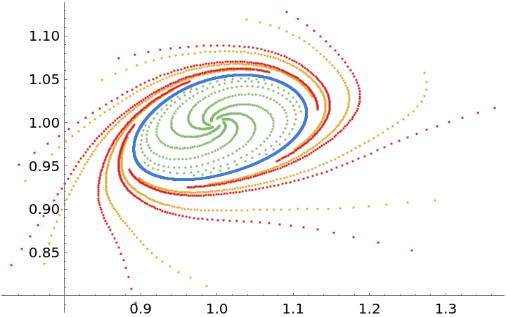
Neimark-Sacker bifurcation (13)
Use IteratedMap2D considering three initial conditions with the following two-dimensional discrete-time dynamical system  :
:
Jacobian matrix:
The non-trivial fixed point:
The Neimark-Sacker critical bifurcation value:
The transversality condition:
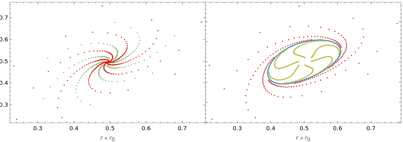
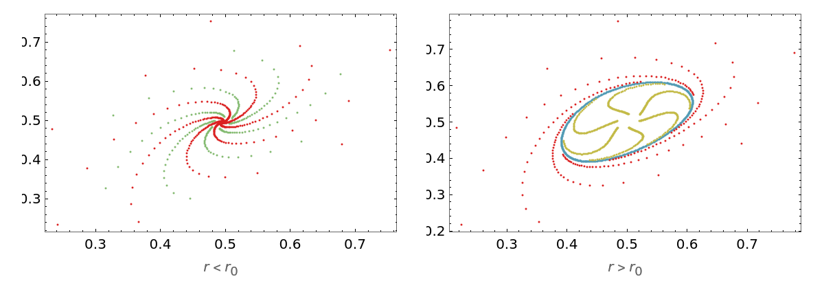
The non-trivial fixed point is unstable for 𝓇>𝓇0 and locally stable for 𝓇<r0, with the stable closed invariant curve bifurcating from  for 𝓇>𝓇0. Define the system for 𝓇<r0 and 𝓇>𝓇0:
Initial conditions for 𝓇<r0 and 𝓇>𝓇0:
Intervals of the maximum number of iterations for 𝓇<r0 and 𝓇>𝓇0:
Step size of iterations for each initial condition when 𝓇<r0 and 𝓇>𝓇0:
Orbits data for 𝓇<r0:
Orbits data for 𝓇>r0:
Visualize the phase portrait graphics for the two conditions:
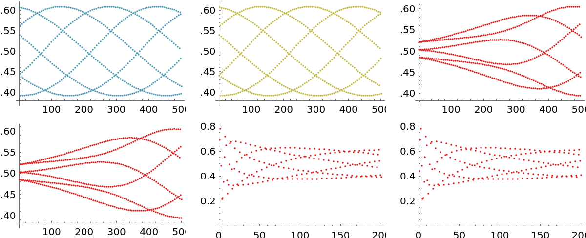
Generate time series data for the discrete-time dynamical system:
Multiple Attractors in a Predator-Prey Model (5)
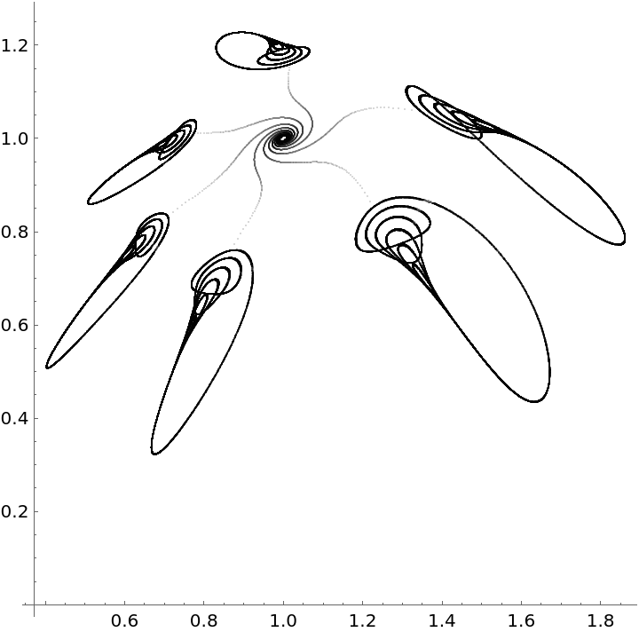
Define a predator-prey model using the Crowley-Martin functional response  and initial conditions:
Interval of the maximum number of iterations for each initial condition:
Step size of iterations for each initial condition:
Orbits data:
Visualize the orbits:
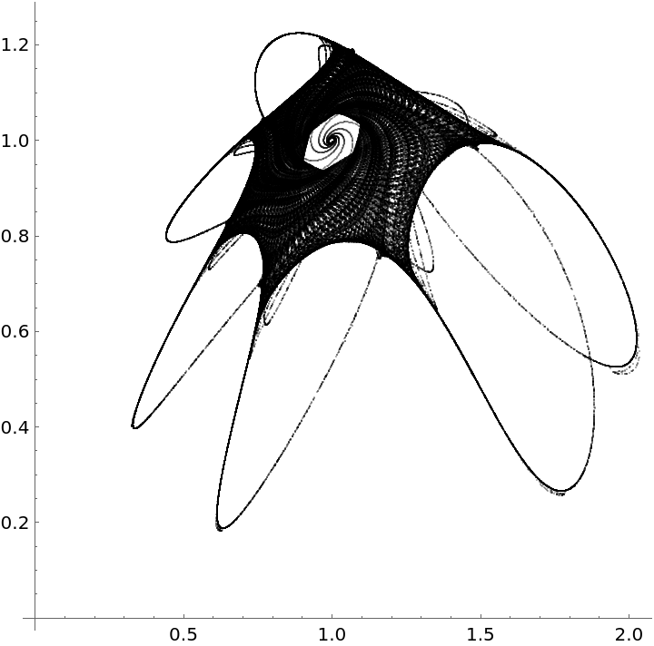
A chaotic attractor:
Interval of the maximum number of iterations:
Step size of iterations for the initial condition X0:
Orbit data:
Visualize the orbit:
First strange attractor:
Orbit data:
Visualize the orbit:
Second strange attractor:
Orbit data:
Visualize the orbit:
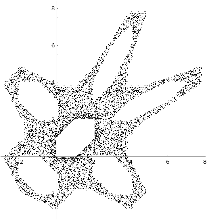
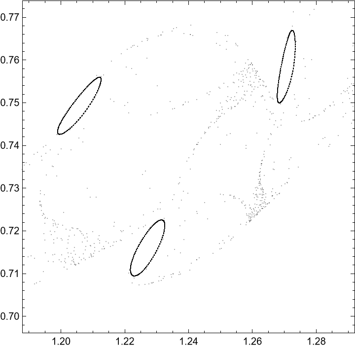
Third strange attractor with multiple periodic orbits:
Initial condition:
Orbit data:
Visualize the orbit:
Zoom into an "interesting" region:
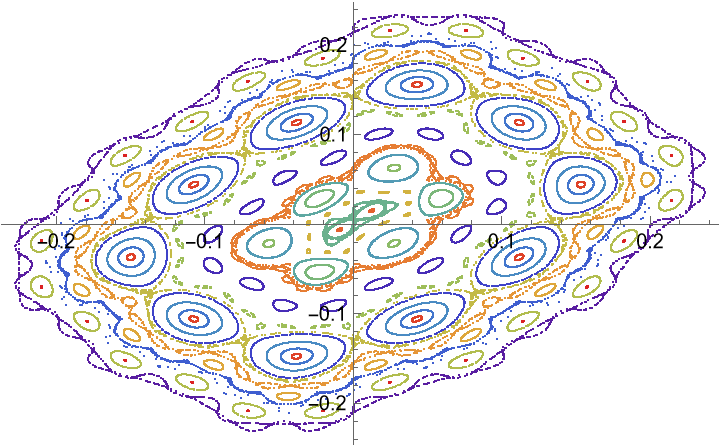
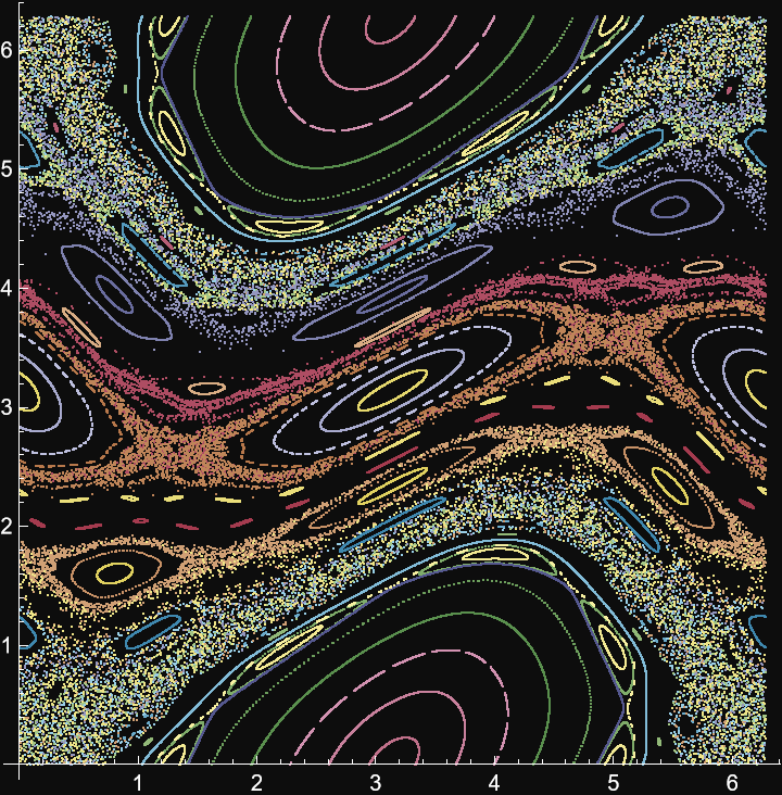
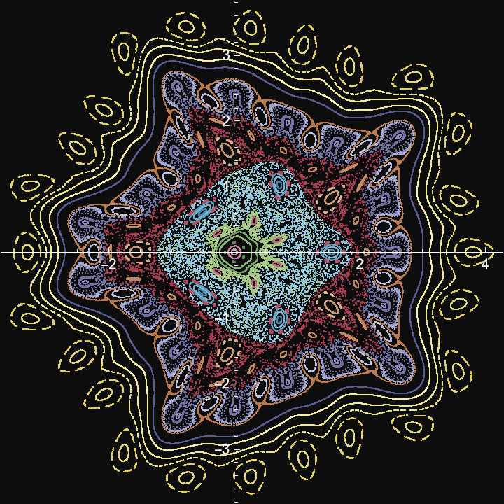
Standard Map (5)
The standard map is defined by the equation 𝓍n+1=𝓍n+ε sin(𝓍n) , 𝓎n+1=𝓎n+𝓍n+1 where 𝓍n and 𝓎n are taken modulo 2π:
Interval of the maximum number of iterations for each initial condition:
Step size of iterations for each initial condition:
Orbits data:
Visualize the orbits:
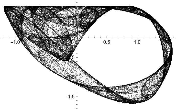
Gumowski-Mira Attractor (5)
The Gumowski-Mira map is defined by 𝓍n+1=𝒷 𝓎n+𝒻(𝓍n) , 𝓎n+1=𝒻(𝓍n+1)-𝓍n, where  :
:
Interval of the maximum number of iterations for each initial condition:
Step size of iterations for each initial condition:
Orbits data:
Visualize the orbits:
Properties and Relations (4)
The map exhibit a Neimark-Sacker bifurcation for 𝓇>𝓇0 at . IteratedMap2D can be used with the resource function PlotGrid to exhibit in a clear fashion a simple bifurcation diagram for the above map:
Orbits data for 𝓇<r0:
Orbits data for 𝓇>r0:
Visualize the bifurcation diagram:
![eqns[{x_[k_], y_[k_]}] := With[{a = 1/13, b = 1/17, c = 1/23}, {x[k + 1] == y[k] - Sign[a*x[k]]*Sqrt[Abs[a b c x[k]*y[k] + c x[k]]], y[k + 1] == a/13 - x[k]}];
X = {x[k], y[k]}](https://www.wolframcloud.com/obj/resourcesystem/images/23d/23dd143c-1980-472f-9134-eaa9091cd932/628e175e6c5898bf.png)


![seqns[{x_[n_], y_[n_]}] := With[{r = 1.98}, {x[n + 1] == r x[n] (1 - y[n]), y[n + 1] == x[n]}];
ueqns[{x_[n_], y_[n_]}] := With[{r = 2.012}, {x[n + 1] == r x[n] (1 - y[n]), y[n + 1] == x[n]}];
X = {x[n], y[n]}](https://www.wolframcloud.com/obj/resourcesystem/images/23d/23dd143c-1980-472f-9134-eaa9091cd932/67fff10eed3b63b4.png)
![{Graphics[
MapIndexed[{PointSize[0.006], ColorData["Rainbow"][#2[[1]]/Length[X0s]], Point[#1]} &, sdata], {Frame -> True, FrameTicksStyle -> GrayLevel[0], FrameLabel -> {
TraditionalForm[r < Subscript[r, 0]], None}, Axes -> False, AspectRatio -> GoldenRatio^(-1)}], Graphics[
MapIndexed[{PointSize[0.006], ColorData["Rainbow"][#2[[1]]/Length[X0u]], Point[#1]} &, udata], {Frame -> True, FrameTicksStyle -> GrayLevel[0], FrameLabel -> {
TraditionalForm[r > Subscript[r, 0]], None}, Axes -> False, AspectRatio -> GoldenRatio^(-1)}]} // GraphicsRow](https://www.wolframcloud.com/obj/resourcesystem/images/23d/23dd143c-1980-472f-9134-eaa9091cd932/056cee668de010e4.png)
![GraphicsGrid[
Partition[
Flatten[MapIndexed[{ListPlot[#1, PlotStyle -> {PointSize[0.01], ColorData["Rainbow"][#2[[1]]/Length[X0u]]}]} &, %]], 3]]](https://www.wolframcloud.com/obj/resourcesystem/images/23d/23dd143c-1980-472f-9134-eaa9091cd932/510cc043c52212e8.png)
![eqns[{x_[n_], y_[n_]}] := With[{a = 24647595988461150985968273113/665860725091715916800000000,
b = 247579691107/12800000000, c = 6400000000/80393230369, d = 323537/40000, k = 2828296/1090611, r = 1414148/323537, \[Gamma] = 323537/60000}, {x[n + 1] == r x[n] (1 - x[n]/k) - (
a x[n]*y[n])/((1 + b x[n]) (1 + c y[n])), y[n + 1] == (\[Gamma] a x[n]*y[n])/((1 + b x[n]) (1 + c y[n])) - d y[n]}];
X0 = {{0.995, 0.995}, {0.995, 0.995}, {0.77, 0.82}, {0.9, 0.77}}](https://www.wolframcloud.com/obj/resourcesystem/images/23d/23dd143c-1980-472f-9134-eaa9091cd932/3e7f34211a5b4792.png)
![eqns[{x_[n_], y_[n_]}] := With[{a = 17275862227/622054400, b = 6883/512, c = 256/2209, d = 55/8, k = 488/189, r = 244/55, \[Gamma] = 55/12}, {x[n + 1] == r x[n] (1 - x[n]/k) - (
a x[n]*y[n])/((1 + b x[n]) (1 + c y[n])), y[n + 1] == (\[Gamma] a x[n]*y[n])/((1 + b x[n]) (1 + c y[n])) - d y[n]}];
X = {x[n], y[n]}](https://www.wolframcloud.com/obj/resourcesystem/images/23d/23dd143c-1980-472f-9134-eaa9091cd932/50f56d240ad380a2.png)

![eqns[{x_[n_], y_[n_]}] := With[{a = 4592791259697/181297792000, b = 152923/12800, c = 6400/48841, d = 261/40, k = 776/301, r = 388/87, \[Gamma] = 87/20}, {x[n + 1] == r x[n] (1 - x[n]/k) - (a x[n]*y[n])/((1 + b x[n]) (1 + c y[n])), y[n + 1] == (\[Gamma] a x[n]*y[n])/((1 + b x[n]) (1 + c y[n])) - d y[n]}]](https://www.wolframcloud.com/obj/resourcesystem/images/23d/23dd143c-1980-472f-9134-eaa9091cd932/76800ca4db0cff1e.png)
![eqns[{x_[n_], y_[n_]}] := With[{a = 8592991153063/334815411200, b = 155587/12800, c = 6400/49729, d = 263/40, k = 2344/909, r = 1172/263, \[Gamma] = 263/60}, {x[n + 1] == r x[n] (1 - x[n]/k) - (a x[n]*y[n])/((1 + b x[n]) (1 + c y[n])), y[n + 1] == (\[Gamma] a x[n]*y[n])/((1 + b x[n]) (1 + c y[n])) - d y[n]}]](https://www.wolframcloud.com/obj/resourcesystem/images/23d/23dd143c-1980-472f-9134-eaa9091cd932/1e445d4e41121bee.png)
![eqns[{x_[n_], y_[n_]}] := With[{a = 24686881771241562225059473113/665860725091715916800000000,
b = 247579691107/12800000000, c = 6400000000/80393230369, d = 323537/40000, k = 2828296/1090611, r = 1414148/323537, \[Gamma] = 323537/60000}, {x[n + 1] == r x[n] (1 - x[n]/k) - (
a x[n]*y[n])/((1 + b x[n]) (1 + c y[n])), y[n + 1] == (\[Gamma] a x[n]*y[n])/((1 + b x[n]) (1 + c y[n])) - d y[n]}];
X = {x[n], y[n]}](https://www.wolframcloud.com/obj/resourcesystem/images/23d/23dd143c-1980-472f-9134-eaa9091cd932/6d5c1cda76d91e45.png)

![StandardMap[{x_[n_], y_[n_]}][\[CurlyEpsilon]_] := {x[n + 1] == Mod[x[n] + y[n] + \[CurlyEpsilon] Sin[x[n]], 2 \[Pi]], y[n + 1] == Mod[y[n] + \[CurlyEpsilon] Sin[x[n]], 2 \[Pi]]};
X0 = {{0.0952, 0.2801}, {2.9067, 4.5882}, {0.6671, 5.8718}, {0.8733, 4.5413}, {0.9015, 1.03502}, {5.8875, 5.6839}, {5.3908, 0.2054}, {1.48266, 0.1584}, {1.6982, 0.1427}, {1.9887, 0.0645}, {2.3261, 0.0801}, {2.6635, 0.0958}, {3.0009, 0.0801}, {5.9812, 5.6842}, {0.1986, 4.0092}, {0.1612, 2.0112}, {1.4451, 3.1748}, {0.1237, 1.646}, {0.4704, 1.6512}, {0.0581, 2.5017}, {1.8856, 2.6791}, {2.148, 2.7313}, {2.551, 2.893}, {0.0581, 4.448}, {0.3673, 4.3436}, {5.3346, 4.6776}, {1.642, 4.8237}, {1.164, 5.8307}, {1.2296, 5.4759}, {0.208, 1.7242}, {0.3673, 2.2147}, {2.9166, 3.0809}, {0.6766, 1.6303}};](https://www.wolframcloud.com/obj/resourcesystem/images/23d/23dd143c-1980-472f-9134-eaa9091cd932/40302ffafe0446d1.png)

![f[x_[n_]][a_] := a x[n] + (2 (1 - a) x[n]^2)/(1 + x[n]^2)^2;
GMAttractor[{x_[n_], y_[n_]}][{a_, b_}] := {x[n + 1] == b y[n] + a x[n] + (2 (1 - a) x[n]^2)/(1 + x[n]^2)^2, y[n + 1] == ReplaceAll[
x[n] -> b y[n] + a x[n] + (2 (1 - a) x[n]^2)/(1 + x[n]^2)^2][
f[x[n]][a]] - x[n]};
X0 = CompressedData["
1:eJwBwQE+/iFib1JlAgAAABsAAAACAAAAmpmZmZmZ2T+amZmZmZnpP3im89iz
m+Q/pJU/eXFZ8D8A0nv1WufkPzbXUirsFPM/aMFoEnKH5j/z+xHTiVTxP6Bd
al/YS9G/hXUPYVefxj9gSs8tzSLJvxRij9pU8rc/uO105ZUw1z/qfuPiMW68
P8CI2ReBAsI/1DYRTok4sT/AQggq7N6ZP7wI/P6Mv6I/gO5KipLBqD/eWnqY
XdO2PyAOF/XqkuM/Gmfl3GhhxD9wPESZBozUv6A6cfTdIek/BE+hRKfV8z9t
fPbEm2npP97QD+C9EvU/VFGZd+Ph6D+2NLWPaS/3P4gIkRSQbug/8InNFKbF
5z/U57zzY4H5P0R5mB7VtgBAonow32bU+D90IQtGnBfyvxjyAfT56PI/WP8E
YwqD4z9k3ou/CqsBQI5FyTBZpgRAfUZjNnez+7+K2HL/SE8FQKih69vvk/q/
EFXx6uZj7z9Mg/MnlfkCwEJI7EwxPvI/8pVS2/rTA8BesHjJA27zPw2ppQJV
CwXAQqcGdOBe9T+CS379GG4GwKrpYsPETv0/gjM36v2cBcDCSx2XAvf/vzRg
qa74owJAZtDkwQ==
"]](https://www.wolframcloud.com/obj/resourcesystem/images/23d/23dd143c-1980-472f-9134-eaa9091cd932/20a3d1e176fae1ae.png)


![Short[sdata1 = ResourceFunction[
"IteratedMap2D", ResourceSystemBase -> "https://www.wolframcloud.com/objects/resourcesystem/api/1.0"][{x[n + 1] == 1.98 x[n] (1 - y[n]), y[n + 1] == x[n]}, X1s, {x[n], y[n]}, {n, {{1, 200}, {1, 500}}}, ConstantArray[1, Length[X1s]]]]](https://www.wolframcloud.com/obj/resourcesystem/images/23d/23dd143c-1980-472f-9134-eaa9091cd932/3a5c3fa2b74bd645.png)
![Short[udata1 = ResourceFunction[
"IteratedMap2D", ResourceSystemBase -> "https://www.wolframcloud.com/objects/resourcesystem/api/1.0"][{x[n + 1] == 2.012 x[n] (1 - y[n]), y[n + 1] == x[n]}, X1u, {x[n], y[n]}, {n, {{1000, 1500}, {1, 500}, {1, 200}}}, ConstantArray[1, Length[X1u]]]]](https://www.wolframcloud.com/obj/resourcesystem/images/23d/23dd143c-1980-472f-9134-eaa9091cd932/61ee1cb7d0cf6b77.png)
![ResourceFunction[
"PlotGrid"][{{Graphics[
MapIndexed[{PointSize[0.006], ColorData["Rainbow"][#2[[1]]/Length[X1s]], Point[#1]} &, sdata1], {Frame -> True, FrameTicksStyle -> GrayLevel[0], FrameLabel -> {
TraditionalForm[r < Subscript[r, 0]], None}, Axes -> False, AspectRatio -> GoldenRatio^(-1)}], Graphics[
MapIndexed[{PointSize[0.006], ColorData["Rainbow"][#2[[1]]/Length[X1u]], Point[#1]} &, udata1], {Frame -> True, FrameTicksStyle -> GrayLevel[0], FrameLabel -> {
TraditionalForm[r > Subscript[r, 0]], None}, Axes -> False, AspectRatio -> GoldenRatio^(-1)}]}}, ImageSize -> 700]](https://www.wolframcloud.com/obj/resourcesystem/images/23d/23dd143c-1980-472f-9134-eaa9091cd932/05ec6d0d5ee14255.png)