Basic Examples (2) 

Invert point P₁={2,2} with respect to the reference unit circle to

In[1]:=

Out[1]=

This is the expected result from the power of a circle r²=1²=OP₁·OP₂

In[2]:=

Out[2]=

Invert a circle to another circle:

In[3]:=

Out[3]=

Scope (2) 

CircleInversion works with arbitrary curves represented in parametric form for symbolic arguments. ParametricPlot can be used to visualize the transformed curve.

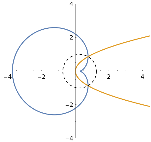
The inversion of a parabola is a cardioid if the center of inversion is the parabola's focus:

In[4]:=

Out[4]=

In[5]:=

Out[5]=

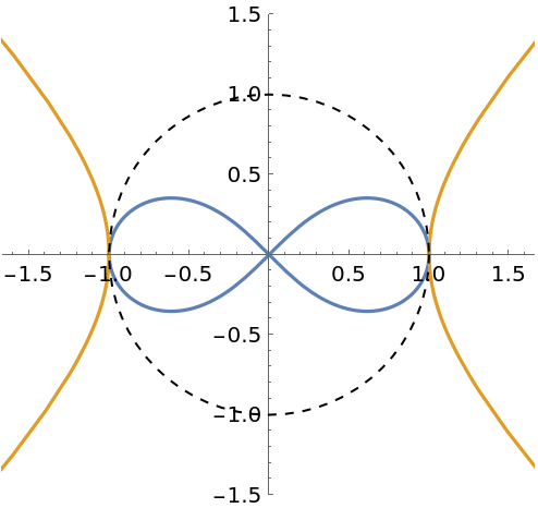
The inversion of an equilateral hyperbola is a lemniscate of Bernoulli if the reference circle is centered on the bisector of the hyperbola's two foci:

In[6]:=

Out[6]=

In[7]:=

Out[7]=

In[8]:=

Out[8]=

Applications (4) 

The inverse of a circle is another circle if the original circle does not contain the center of inversion:

In[9]:=

Out[9]=

The inverse of a circle is a line if the original circle contains the center of inversion:

In[10]:=

Out[10]=

The inverse of a line is a circle containing the center of inversion if the line does not contain the center:

In[11]:=

Out[11]=

A line inverts to itself if it contains the center of inversion:

In[12]:=

Out[12]=

Properties and Relations (3) 

CircleInversion is its own inverse:

In[13]:=

Out[13]=

In[14]:=

Out[14]=

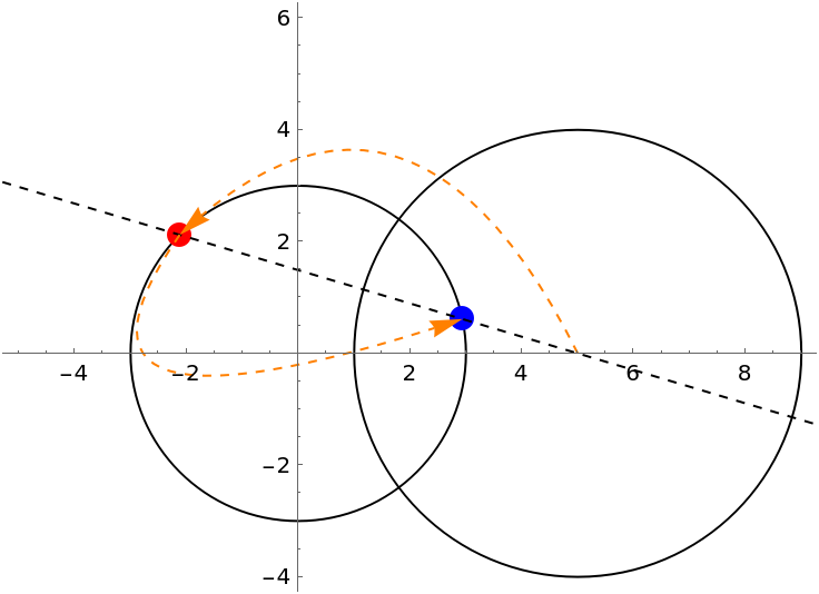
Orthogonal circles are invariant under inversion with respect to each other. However, every point on each circle is inverted to a different place on the same circle (except for the intersection points):

In[15]:=

Out[15]=

In[16]:=

Out[16]=

For instance, the point (red) is on the Circle[{0,0},3], which is inverted to the different location (blue) on the same circle:

In[17]:=

Out[17]=

In[18]:=

Out[18]=

Its distance from the origin is still 3:

In[19]:=

Out[19]=

Regardless of the different types of objects returned by this function, the result of CircleInversion is in general closed under a set of objects recognized by Graphics:

In[20]:=

Out[20]=

Possible Issues (4) 

The inverse of the center of the reference circle is defined as Infinity:

In[21]:=

Out[21]=

Conversely, the inverse of Infinity is the inversion center:

In[22]:=

Out[22]=

CircleInversion does not distinguish between Line and InfiniteLine in the second argument:

In[23]:=

Out[23]=

In[24]:=

Out[24]=

CircleInversion returns different results based on the syntax of InfiniteLine.

For an infinite line that goes through {3,1} and {1,0}, which does not include the inversion center, its image is a circle containing the inversion center:

In[25]:=

Out[25]=

For an infinite line that passes through {3,1} and is in the same direction as the vector {1,0} (a horizontal line that passes through the inversion center), its image is the line itself:

In[26]:=

Out[26]=

In general, the center of the original circle and that of its inversion are not inversion points with respect to each other:

In[27]:=

Out[27]=

In[28]:=

Out[28]=

The center of the image is the midpoint of the inversion of the antipodal points on the original circle:

In[29]:=

Out[29]=

In[30]:=

Out[30]=

Neat Examples (3) 

Let three circles have a common point. Suppose that the common chord of two of them is a diameter of the third. If this is true for two of the three common chords, then you can prove it must be true for all three of them (C. S. Ogilvy, Excursions in Geometry).

Proof by inversion: Convert the diagram on the left to right, complete the proof with the concurrency of three altitudes in any triangle. The center of inversion is the concurrency of three circles.

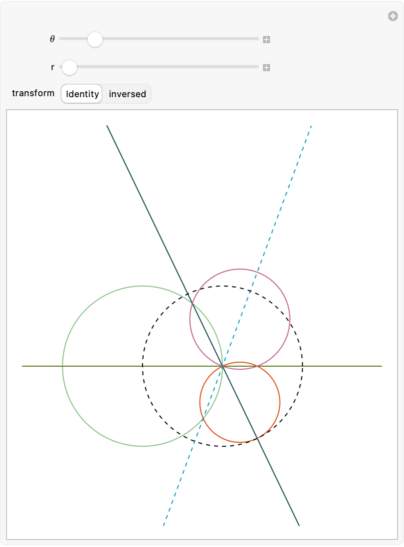
Use Manipulate to see the invariance of the result by changing the configuration of the circles constrained by the statement of the problem:

In[31]:=

Out[32]=

Semicircles with centers at A (red) and B (blue) and with radii 2 and 1, respectively, are drawn in the interior of, and sharing bases with, a semicircle with diameter JK. The two smaller semicircles are externally tangent to each other and internally tangent to the largest semicircle (dashed). A circle centered at P is drawn externally tangent to the two smaller semicircles and internally tangent to the largest semicircle. What is the radius of the circle centered at P? (2017 AMC 12A Problem 16)

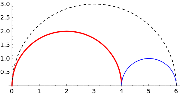
Here is the Arbelos and Chain of Pappus:

In[33]:=

Out[34]=

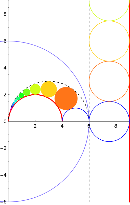
The result can be easily generalized to the n^th circle in the chain by circle inversion. Choose the center of inversion to be {0,0} and let the radius of the reference circle be 6 ( marked by as the largest circle in the diagram at bottom):

In[35]:=

Out[36]=

Find the radius of the first fifteen circles in the chain:

In[37]:=

Out[38]=

In[39]:=

Out[39]=

In[40]:=

Out[40]=

The framed part is the answer to this problem. In the diagram below, each disk is the element in the chain of Pappus by inverting the circle with the same color from the column on the right:

In[41]:=

Out[42]=

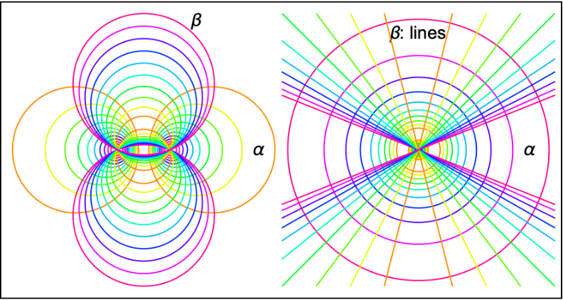
The combination of inversion and a coaxial family (or pencil of circles) is the key step to finding the Steiner chain of two given non-intersecting circles. For 0<|t|<1, one has the points , B={t,0}, C={1,0} and D={-1,0}. Then A and B are harmonic conjugates with respect to C and D. Define the α and β families of circles:

In[43]:=

Out[44]=

In[45]:=

Out[46]=

Any pair of circles, one from each family, intersects orthogonally:

In[47]:=

Out[47]=

Check the dot product of two vectors which sit at each center of the circles and point to the intersection:

In[48]:=

Out[48]=

This also proves that the locus of the center of circles in the β family (or the perpendicular bisector of segment CD) is the radical axis for any two circles in the α family.

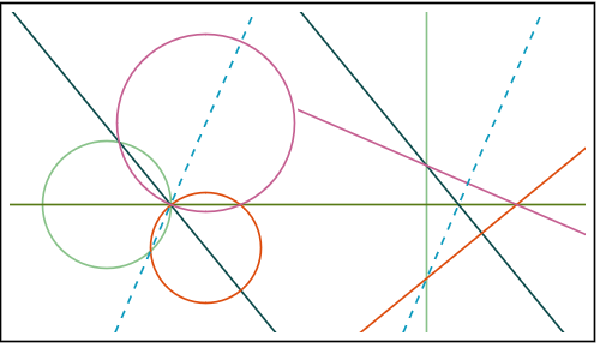
The circles in both coaxial families can be inverted with respect to the reference circle centered at point C:

In[49]:=

Out[50]=

In[51]:=

Out[51]=

In[52]:=

Out[52]=

In[53]:=

Out[53]=

The β circles contain the inversion center, and they are thus mapped to lines. The inverses of the α circles are circles, and they must orthogonally intersect the inverses of the β circles. This is due to the anti-conformal property of circle inversion. The only possibility is that the inverse of the α circles are concentric circles with the common center at point C:

In[54]:=

Out[55]=

The result implies that one only needs to consider the case of concentric circles to determine the number of circles in a closed Steiner chain. This number is invariant under inversion.