Wolfram Function Repository
Instant-use add-on functions for the Wolfram Language
Function Repository Resource:
Implementation of the BusyBoxes 3D reversible cellular automaton
ResourceFunction["BusyBoxesAutomaton"][init] runs the BusyBoxes cellular automaton rule starting from an initial 3D state init. | |
ResourceFunction["BusyBoxesAutomaton"][init,n] runs for n steps. | |
ResourceFunction["BusyBoxesAutomaton"][init,-n] runs for n steps in reverse. | |
ResourceFunction["BusyBoxesAutomaton"][init,n,phase] runs with an initial integer phase. | |
ResourceFunction["BusyBoxesAutomaton"][state,"Swaps", phase] return an explicit list of swap rules for a single step starting from a state with an optional phase. | |
ResourceFunction["BusyBoxesAutomaton"][state,"Visualization"] return a 3D visualization for a state. | |
ResourceFunction["BusyBoxesAutomaton"][arguments][state] represents an operator form. |

Run BusyBoxesAutomaton starting from a random initial condition for a single step:
| In[1]:= |
| Out[1]= |
Run BusyBoxesAutomaton for 3 steps and visualize it:
| In[2]:= | ![ResourceFunction["BusyBoxesAutomaton"]["Visualization"] /@ ResourceFunction["BusyBoxesAutomaton"][
RandomChoice[{.9, .1} -> {0, 1}, {6, 6, 6}], 3]](https://www.wolframcloud.com/obj/resourcesystem/images/68d/68d56c25-e6c9-4c3c-a71d-8c52c9c7de46/1-0-0/2cd91bf5ef70bfea.png) |
| Out[2]= | 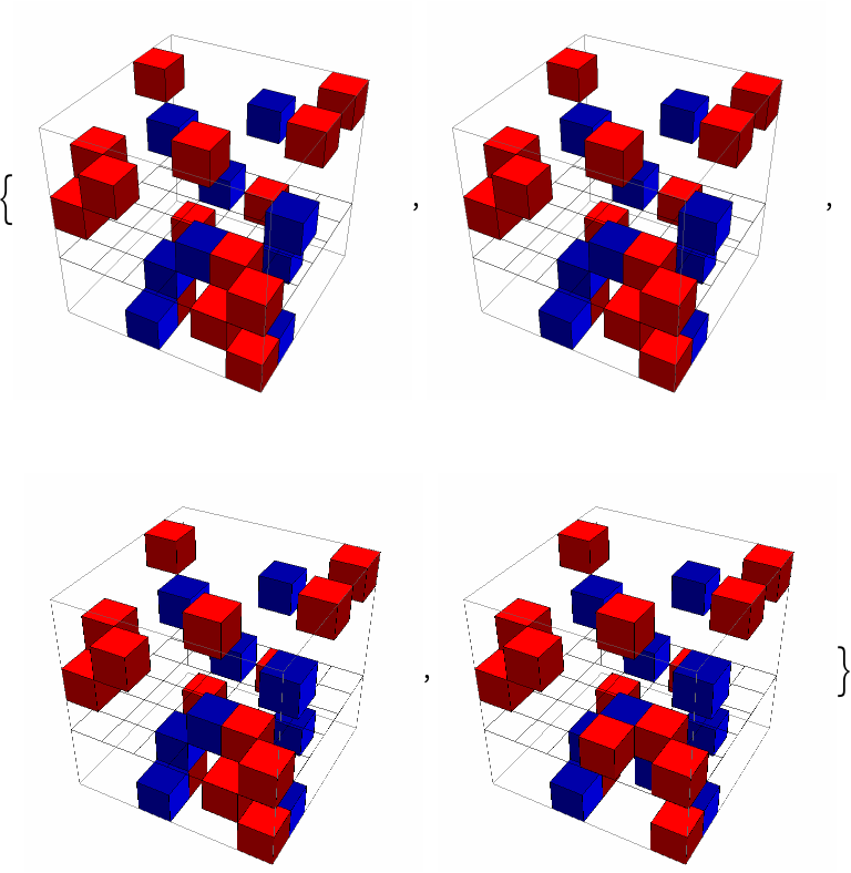 |
Run BBX for 100 steps and 100 more in reverse:
| In[3]:= | ![ListAnimate[
ResourceFunction["BusyBoxesAutomaton"][
"Visualization"] /@ (Join[#, ResourceFunction["BusyBoxesAutomaton"][Last[#], -100]] &@
ResourceFunction["BusyBoxesAutomaton"][
SparseArray[{{7, 4, 4} -> 1, {5, 5, 4} -> 1, {7, 3, 6} -> 1}, {10, 10, 10}], 100]), SaveDefinitions -> True]](https://www.wolframcloud.com/obj/resourcesystem/images/68d/68d56c25-e6c9-4c3c-a71d-8c52c9c7de46/1-0-0/624f1dd0b0e55889.png) |
| Out[3]= | 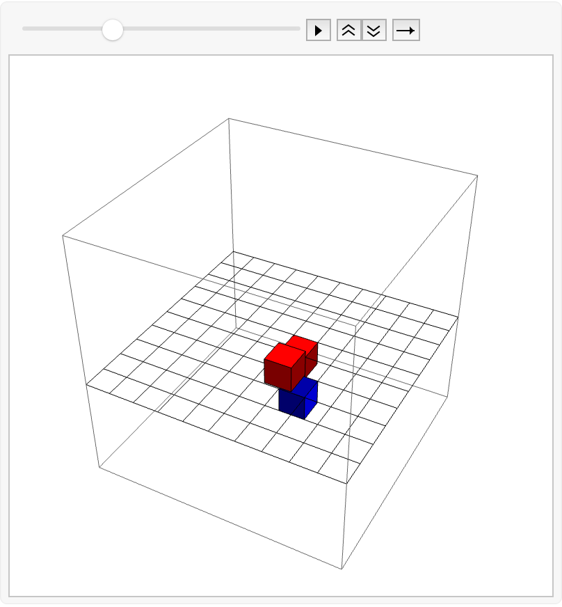 |
Gliders:
| In[4]:= | ![glider1 = SparseArray[{{11, 12, 12} -> 1, {13, 13, 12} -> 1}, {24, 24, 24}];
glider2 = SparseArray[{{12, 11, 14} -> 1, {13, 13, 14} -> 1, {14, 15, 14} -> 1, {15, 17, 14} -> 1}, {24, 24, 24}];
glider3 = SparseArray[{{14, 9, 16} -> 1, {14, 11, 16} -> 1, {13, 11, 16} -> 1, {13, 13, 16} -> 1, {19, 19, 16} -> 1}, {24, 24, 24}];
glider4 = SparseArray[{{15, 9, 18} -> 1, {14, 9, 18} -> 1, {14, 11, 18} -> 1, {13, 11, 18} -> 1, {13, 13, 18} -> 1}, {24, 24, 24}];](https://www.wolframcloud.com/obj/resourcesystem/images/68d/68d56c25-e6c9-4c3c-a71d-8c52c9c7de46/1-0-0/0a4b999ac6c38605.png) |
| In[5]:= | ![ListAnimate[
ResourceFunction["BusyBoxesAutomaton"]["Visualization"] /@ ResourceFunction["BusyBoxesAutomaton"][glider3, 1000], SaveDefinitions -> True]](https://www.wolframcloud.com/obj/resourcesystem/images/68d/68d56c25-e6c9-4c3c-a71d-8c52c9c7de46/1-0-0/6264c047683afef8.png) |
| Out[5]= | 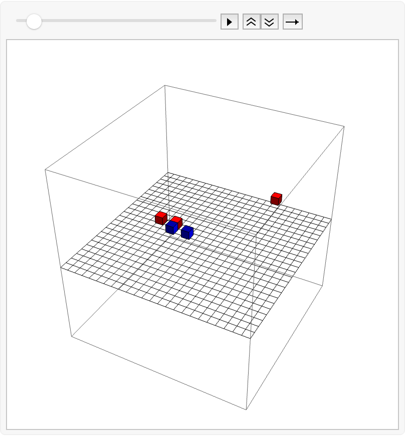 |
| In[6]:= | ![makeBBCircularMotion[n : _Integer?Positive : 3, size_Integer : 40] := Block[{c = Quotient[size, 2], start}, start = {c + 2, c - 2, c + 2};
SparseArray[
Thread[Append[
FoldList[Plus, start, Take[Catenate@Table[{{0, 1, -2}, {0, 2, -1}}, Ceiling[n/2]], n]], start + {-2, -1, 0}] -> 1], ConstantArray[size, 3]]
]](https://www.wolframcloud.com/obj/resourcesystem/images/68d/68d56c25-e6c9-4c3c-a71d-8c52c9c7de46/1-0-0/50cd32eccbd924b9.png) |
| In[7]:= | ![Dynamic[Show[
ResourceFunction["BusyBoxesAutomaton"][state, "Visualization"], If[ListQ[traces], Graphics3D[{Green, Point /@ Mean /@ traces}], Nothing]]]](https://www.wolframcloud.com/obj/resourcesystem/images/68d/68d56c25-e6c9-4c3c-a71d-8c52c9c7de46/1-0-0/059df9a97baf7e20.png) |
| Out[7]= | 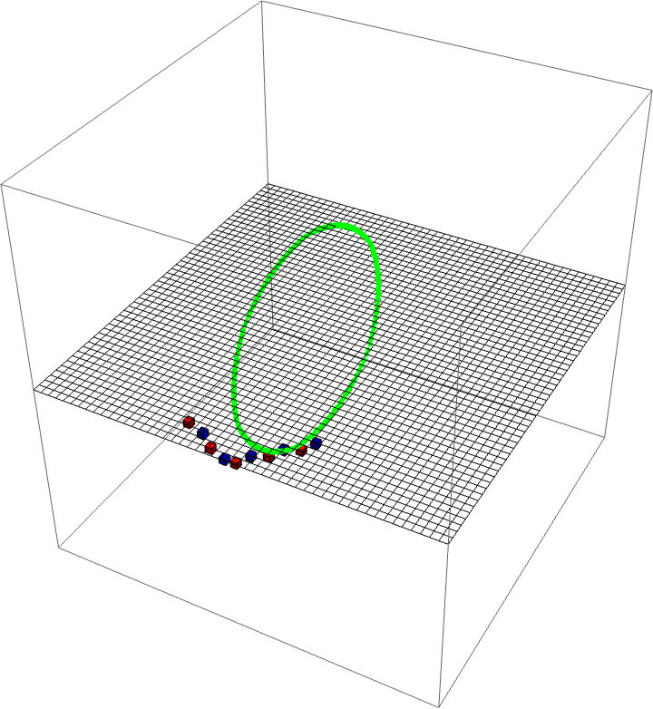 |
Implement code for tracking circular motion:
| In[8]:= | ![states = {};
state = makeBBCircularMotion[8, 50];
traces = {state["ExplicitPositions"]};
phase = 0;
step = 0;
While[step < 1000,
(*Pause[0.01];*)
positions = state["ExplicitPositions"];
AppendTo[states, state];
swaps = ResourceFunction["BusyBoxesAutomaton"][state, "Swaps", phase];
state = SparseArray @ ReplacePart[Normal[state], Catenate @ swaps];
swaps = Cases[swaps, Except[{_ -> 0, _ -> 0}]][[All, All, 1]];
swapRules = With[{pos = FirstPosition[swaps, #, Missing[], {2}, Heads -> False]}, # -> If[MissingQ[pos], #, First@DeleteElements[Extract[swaps, Drop[pos, -1]], {#}]]] & /@
positions;
AppendTo[traces, Replace[traces[[-1]], swapRules, {1}]];
phase = Mod[phase + 1, 6];
step++
]](https://www.wolframcloud.com/obj/resourcesystem/images/68d/68d56c25-e6c9-4c3c-a71d-8c52c9c7de46/1-0-0/685f1959dd172ded.png) |
Show the circular motion:
| In[9]:= | ![Show[ResourceFunction["BusyBoxesAutomaton"][#, "Visualization", "Grid" -> False] & /@ states, Graphics3D[{Green, Point /@ Mean /@ traces}]]](https://www.wolframcloud.com/obj/resourcesystem/images/68d/68d56c25-e6c9-4c3c-a71d-8c52c9c7de46/1-0-0/6bc13f9a16c14cb7.png) |
| Out[9]= | 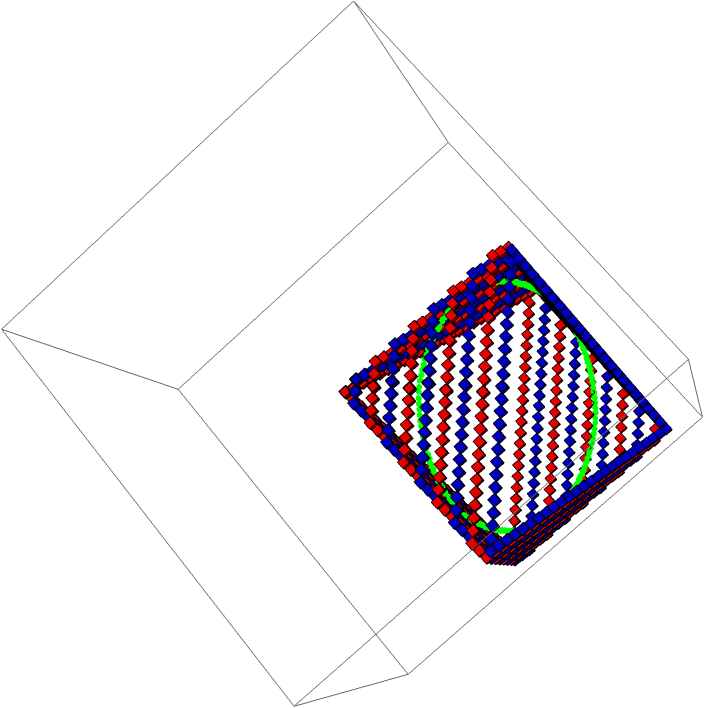 |
This work is licensed under a Creative Commons Attribution 4.0 International License