Details
Possible forms for rule are:
| {in1→out1,in2→out2,…} | a list of rules |
| Dispatch[{in1→out1,…}] | an optimized list of rules |
| Association[in1→out1,…] | a lookup dictionary |
| {rule, dim} | with rule any of the above, and dim equals block length |
Specification by
Association may lead to the fastest calculations, but it requires a comprehensive list of inputs without any usage of pattern matching or
RuleDelayed. Lists of rules may lead to slightly slower calculations, but are more flexible by allowing for pattern matching. The
Dispatch usage should not be much slower than the
Association usage.
ResourceFunction["BlockCellularAutomaton"] allows one extra rule specification {rule,{2,2}} for evolutions through two spatial dimensions, which alternate between phase values 0 and 1 with {2,2} block offset along the diagonal. This is sometimes referred to as the "Margolus neighborhood". More algorithm design regarding phases and offsets remains to be done to implement full dimensional generalization of ResourceFunction["BlockCellularAutomaton"].
Possible forms for time t are:
| t | all steps 0 through t |
| {t} | a list containing only step t |
| {{t}} | step t alone |
| {t1,t2} | steps t1 through t2 |
| {t1,t2,dt} | steps t1,t1+dt, … |
List items in the output of
ResourceFunction["BlockCellularAutomaton"] take the form {
statei,
phasei}, where
phase goes from
0,1,…,dim-1 and
dim is the fixed block length. To obtain an
ArrayPlot of a time evolution, simply discard
phase information by combining
Map and
First, as in examples given below.
The length of init should be commensurate with the block size dim.
Previous versions of this code used a different phase convention, phase ∈{1,2,…, dim}. Backward-compatible usage expects a phase in the previous convention and automatically subtracts one to convert to the present convention.
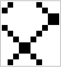
![ArrayPlot[
Map[First, ResourceFunction[
"BlockCellularAutomaton", ResourceSystemBase -> "https://www.wolframcloud.com/obj/resourcesystem/api/1.0"][{
{0, 0} -> {0, 0}, {0, 1} -> {1, 0}, {1, 0} -> {0, 1}, {1, 1} -> {1, 1}
}, {Normal[SparseArray[{2 -> 1, 7 -> 1}, 10]], 0}, 10]], ImageSize -> 100]](https://www.wolframcloud.com/obj/resourcesystem/images/67f/67fa78cf-815d-40ba-85cc-918b434275ac/393e126b4fb4199c.png)
![ResourceFunction[
"BlockCellularAutomaton", ResourceSystemBase -> "https://www.wolframcloud.com/obj/resourcesystem/api/1.0"][{{0, 0, 0} -> {0, 0, 1}, {0, 0, 1} -> {0, 1, 1}, {0, 1, 0} -> {1, 0, 1}, {0, 1, 1} -> {0, 0, 0}, {1, 0, 0} -> {1, 1, 0}, {1, 0, 1} -> {1, 0, 0}, {1, 1, 0} -> {0, 1, 0}, {1, 1, 1} -> {1, 1, 1}},
{Normal[SparseArray[{2 -> 1, 7 -> 1}, 12]], 0}]](https://www.wolframcloud.com/obj/resourcesystem/images/67f/67fa78cf-815d-40ba-85cc-918b434275ac/42637d88a0ba27f7.png)
![ResourceFunction[
"BlockCellularAutomaton", ResourceSystemBase -> "https://www.wolframcloud.com/obj/resourcesystem/api/1.0"][
Dispatch[{{1, 1} -> {2, 0}, {1, 2} -> {2, 1}, {2, 0} -> {1, 1}, {2, 1} -> {1, 2}, {0, 0} -> {0, 0}, {0, 2} -> {0, 2}, {1, 0} -> {1, 0}, {2, 2} -> {2, 2}, {0, 1} -> {1, 1}}],
{CenterArray[{2, 2}, 100], 0}, {{100}}]](https://www.wolframcloud.com/obj/resourcesystem/images/67f/67fa78cf-815d-40ba-85cc-918b434275ac/56b52524948689c3.png)

![Apply[ResourceFunction[
"BlockCellularAutomaton", ResourceSystemBase -> "https://www.wolframcloud.com/obj/resourcesystem/api/1.0"][Association[
{{1, 1} -> {0, 0}, {1, 0} -> {1, 0}, {0, 1} -> {0, 1}, {0, 0} -> {1, 1}}]],
{{1, 1, 0, 1, 0, 0}, 0}]](https://www.wolframcloud.com/obj/resourcesystem/images/67f/67fa78cf-815d-40ba-85cc-918b434275ac/48a3764715acc9a9.png)
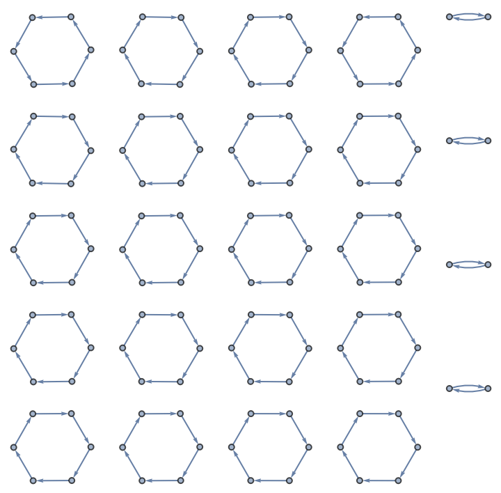
![With[{caOperator = ResourceFunction[
"BlockCellularAutomaton", ResourceSystemBase -> "https://www.wolframcloud.com/obj/resourcesystem/api/1.0"][
{{1, 1} -> {0, 0}, {1, 0} -> {1, 0}, {0, 1} -> {0, 1}, {0, 0} -> {1, 1}}]},
Graph[Map[# -> caOperator @@ # &,
Tuples[{Tuples[{1, 0}, 6], {0, 1}}]]]]](https://www.wolframcloud.com/obj/resourcesystem/images/67f/67fa78cf-815d-40ba-85cc-918b434275ac/2df12ade496bc186.png)
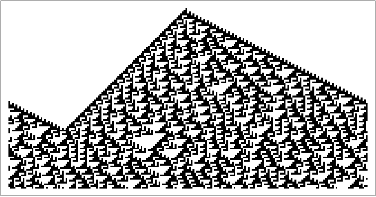
![ArrayPlot[Map[RotateRight[First[#], 30] &,
ResourceFunction[
"BlockCellularAutomaton", ResourceSystemBase -> "https://www.wolframcloud.com/obj/resourcesystem/api/1.0"][{{{x_, y_, z_} :> {
Mod[(x - z), 3], Mod[(y - x), 3], Mod[(z - y), 3]
}}, 3}, {CenterArray[{1}, 201], 3}, 120]]]](https://www.wolframcloud.com/obj/resourcesystem/images/67f/67fa78cf-815d-40ba-85cc-918b434275ac/38da0b6b7310f938.png)

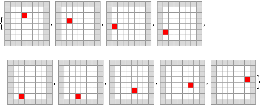
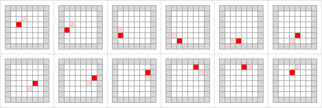
![With[{config = ArrayPad[ReplacePart[
ConstantArray[0, {6, 6}], {2, 3} -> 1], 1, 2]},
ArrayPlot[First[#],
ColorRules -> {0 -> White, 1 -> Red, 2 -> LightGray},
Frame -> None, Mesh -> True,
ImageSize -> 80] & /@
ResourceFunction[
"BlockCellularAutomaton", ResourceSystemBase -> "https://www.wolframcloud.com/obj/resourcesystem/api/1.0"][{
Dispatch[{Condition[{{
Pattern[a,
Blank[]],
Pattern[b,
Blank[]]}, {
Pattern[c,
Blank[]],
Pattern[d,
Blank[]]}},
Or[Count[{a, b, c, d}, 2] == 3,
And[Count[{a, b, c, d}, 2] == 2, Count[{a, b, c, d}, 1] != 1]]] :> {{a, b}, {c, d}}, Condition[{{
Pattern[a,
Blank[]],
Pattern[b,
Blank[]]}, {
Pattern[c,
Blank[]],
Pattern[d,
Blank[]]}},
And[Count[{a, b, c, d}, 2] == 2, Count[{a, b, c, d}, 1] == 1]] :> ReplaceAll[{{a, b}, {c, d}}, {1 -> 0, 0 -> 1}], Condition[{{
Pattern[a,
Blank[]],
Pattern[b,
Blank[]]}, {
Pattern[c,
Blank[]],
Pattern[d,
Blank[]]}},
And[Count[{a, d}, 2] == 1, Count[{b, c}, 2] == 0]] :> {{a, c}, {b, d}},
Condition[{{
Pattern[a,
Blank[]],
Pattern[b,
Blank[]]}, {
Pattern[c,
Blank[]],
Pattern[d,
Blank[]]}},
And[Count[{a, d}, 2] == 0, Count[{b, c}, 2] == 1]] :> {{d, b}, {c, a}}, {{0, 0}, {0, 0}} -> {{0, 0}, {0, 0}}, {{1, 0}, {0, 0}} -> {{0, 0}, {0, 1}}, {{0, 1}, {0, 0}} -> {{0, 0}, {1, 0}}, {{0, 0}, {1, 0}} -> {{0, 1}, {0, 0}}, {{0, 0}, {0, 1}} -> {{1, 0}, {0, 0}}, {{1, 1}, {0, 0}} -> {{0, 0}, {1, 1}}, {{1, 0}, {1, 0}} -> {{0, 1}, {0, 1}}, {{1, 0}, {0, 1}} -> {{0, 1}, {1, 0}}, {{0, 1}, {1, 0}} -> {{1, 0}, {0, 1}}, {{0, 1}, {0, 1}} -> {{1, 0}, {1, 0}}, {{0, 0}, {1, 1}} -> {{1, 1}, {0, 0}}, {{1, 1}, {1, 0}} -> {{0, 1}, {1, 1}}, {{1, 1}, {0, 1}} -> {{1, 0}, {1, 1}}, {{1, 0}, {1, 1}} -> {{1, 1}, {0, 1}}, {{0, 1}, {1, 1}} -> {{1, 1}, {1, 0}}, {{1, 1}, {1, 1}} -> {{1, 1}, {1, 1}}}], {2, 2}},
{config, 0}, 8]]](https://www.wolframcloud.com/obj/resourcesystem/images/67f/67fa78cf-815d-40ba-85cc-918b434275ac/59d8e02b5cc68aa5.png)

![ResourceFunction[
"BlockCellularAutomaton", ResourceSystemBase -> "https://www.wolframcloud.com/obj/resourcesystem/api/1.0"][
# -> CellularAutomaton[110][#] & /@ Tuples[{1, 0}, 3],
RotateLeft@CenterArray[{1}, 201], 100, 3] // ArrayPlot](https://www.wolframcloud.com/obj/resourcesystem/images/67f/67fa78cf-815d-40ba-85cc-918b434275ac/19b8277b57a4760f.png)
![ResourceFunction[
"BlockCellularAutomaton", ResourceSystemBase -> "https://www.wolframcloud.com/obj/resourcesystem/api/1.0"][{
{x_, y_} :> {y, x},
{x_, y_, z_} :> {z, y, x}
}, {IntegerDigits[1009400, 2], 0}, 20]](https://www.wolframcloud.com/obj/resourcesystem/images/67f/67fa78cf-815d-40ba-85cc-918b434275ac/30487b46d4c53b24.png)
![With[{data = Map[First, Last[
ResourceFunction["FindNestedTransientRepeat"][
ResourceFunction[
"BlockCellularAutomaton", ResourceSystemBase -> "https://www.wolframcloud.com/obj/resourcesystem/api/1.0"][{
Dispatch[{Condition[{{
Pattern[a,
Blank[]],
Pattern[b,
Blank[]]}, {
Pattern[c,
Blank[]],
Pattern[d,
Blank[]]}},
Or[Count[{a, b, c, d}, 2] == 3,
And[Count[{a, b, c, d}, 2] == 2, Count[{a, b, c, d}, 1] != 1]]] :> {{a, b}, {c, d}}, Condition[{{
Pattern[a,
Blank[]],
Pattern[b,
Blank[]]}, {
Pattern[c,
Blank[]],
Pattern[d,
Blank[]]}},
And[Count[{a, b, c, d}, 2] == 2, Count[{a, b, c, d}, 1] == 1]] :> ReplaceAll[{{a, b}, {c, d}}, {1 -> 0, 0 -> 1}], Condition[{{
Pattern[a,
Blank[]],
Pattern[b,
Blank[]]}, {
Pattern[c,
Blank[]],
Pattern[d,
Blank[]]}},
And[Count[{a, d}, 2] == 1, Count[{b, c}, 2] == 0]] :> {{a, c}, {b, d}},
Condition[{{
Pattern[a,
Blank[]],
Pattern[b,
Blank[]]}, {
Pattern[c,
Blank[]],
Pattern[d,
Blank[]]}},
And[Count[{a, d}, 2] == 0, Count[{b, c}, 2] == 1]] :> {{d, b}, {c, a}}, {{0, 0}, {0, 0}} -> {{0, 0}, {0, 0}}, {{1, 0}, {0,
0}} -> {{0, 0}, {0, 1}}, {{0, 1}, {0, 0}} -> {{0, 0}, {
1, 0}}, {{0, 0}, {1, 0}} -> {{0, 1}, {0, 0}}, {{0, 0}, {
0, 1}} -> {{1, 0}, {0, 0}}, {{1, 1}, {0, 0}} -> {{0, 0}, {1, 1}}, {{1, 0}, {1, 0}} -> {{0, 1}, {0, 1}}, {{1, 0}, {0, 1}} -> {{0, 1}, {1, 0}}, {{0, 1}, {1, 0}} -> {{1,
0}, {0, 1}}, {{0, 1}, {0, 1}} -> {{1, 0}, {1, 0}}, {{0, 0}, {1, 1}} -> {{1, 1}, {0, 0}}, {{1, 1}, {1, 0}} -> {{0,
1}, {1, 1}}, {{1, 1}, {0, 1}} -> {{1, 0}, {1, 1}}, {{1, 0}, {1, 1}} -> {{1, 1}, {0, 1}}, {{0, 1}, {1, 1}} -> {{1,
1}, {1, 0}}, {{1, 1}, {1, 1}} -> {{1, 1}, {1, 1}}}], {2,
2}}] @@ # &,
{ArrayPad[ReplacePart[ConstantArray[0, {6, 6}],
{2, 3} -> 1], 1, 2], 0}, 5]]]},
Grid[Partition[Map[ArrayPlot[ReplacePart[Last[#],
Position[First[#], 1][[1]] -> -1],
ColorRules -> {0 -> White, 1 -> Red, -1 -> LightRed, 2 -> LightGray},
Frame -> None, Mesh -> True, ImageSize -> 80] &,
Partition[data, 2, 1, 1]], 6],
Frame -> All, FrameStyle -> LightGray,
Spacings -> {1, 1}]]](https://www.wolframcloud.com/obj/resourcesystem/images/67f/67fa78cf-815d-40ba-85cc-918b434275ac/32316c877041e535.png)
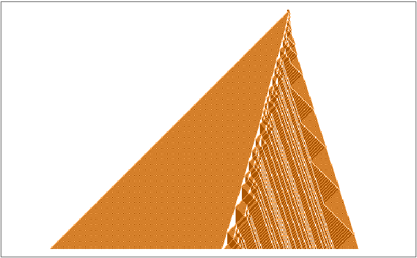
![ArrayPlot[Map[RotateRight[First[#], 100] &,
ResourceFunction[
"BlockCellularAutomaton", ResourceSystemBase -> "https://www.wolframcloud.com/obj/resourcesystem/api/1.0"][
Association[{{0, 0} -> {0, 0}, {0, 1} -> {1, 1},
{0, 2} -> {0, 2}, {1, 0} -> {1, 0}, {1, 1} -> {2, 0},
{1, 2} -> {2, 1}, {2, 0} -> {1, 1}, {2, 1} -> {1, 2},
{2, 2} -> {2, 2}}], {CenterArray[{2, 2}, 500], 0}, 300]], ImageSize -> 300, ColorRules -> {0 -> White, 1 -> Lighter[Orange], 2 -> Darker[Orange]}]](https://www.wolframcloud.com/obj/resourcesystem/images/67f/67fa78cf-815d-40ba-85cc-918b434275ac/47faac7344816529.png)
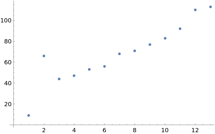
![With[
{data = Map[First, ResourceFunction[
"BlockCellularAutomaton", ResourceSystemBase -> "https://www.wolframcloud.com/obj/resourcesystem/api/1.0"][
Association[{{0, 0} -> {0, 0}, {0, 1} -> {1, 1},
{0, 2} -> {0, 2}, {1, 0} -> {1, 0}, {1, 1} -> {2, 0},
{1, 2} -> {2, 1}, {2, 0} -> {1, 1}, {2, 1} -> {1, 2},
{2, 2} -> {2, 2}}],
{CenterArray[{2, 2}, 2 #], 0}, #]] &@1000},
ListPlot[Differences[MapIndexed[If[
MatchQ[#1, {__, 1, 1, 1, 1, 0 ..}],
#2[[1]], Nothing] &, data]]]]](https://www.wolframcloud.com/obj/resourcesystem/images/67f/67fa78cf-815d-40ba-85cc-918b434275ac/4a1c16b8665684c9.png)
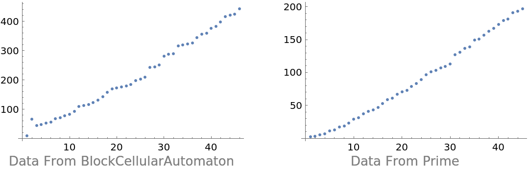
![Grid[{Show[#, ImageSize -> 250] & /@ {
ListPlot[{9, 66, 44, 47, 53, 56, 68, 71, 77, 83, 92, 110, 113, 116, 122, 131, 143, 158, 170, 173, 176, 179, 185, 197, 203, 209, 242, 245, 251, 281, 287, 290, 317, 320, 323, 326, 344, 356, 359, 377, 383, 398, 416, 422, 425, 443}], ListPlot[Prime /@ Range[45]]},
Text[Style[#, Gray]] & /@ {
"Data From BlockCellularAutomaton",
"Data From Prime"}}, Spacings -> {3, 0}]](https://www.wolframcloud.com/obj/resourcesystem/images/67f/67fa78cf-815d-40ba-85cc-918b434275ac/6cb65b7dae155caf.png)
![ArrayPlot[
First /@ ResourceFunction[
"BlockCellularAutomaton", ResourceSystemBase -> "https://www.wolframcloud.com/obj/resourcesystem/api/1.0"][{{2, 2} -> {1, 1}, {1, 1} -> {2, 2}, {1, 2} -> {1, 2}, {2, 1} -> {2, 1}, {2, 0} -> {0, 2}, {1, 0} -> {1, 0}, {0, 2} -> {2, 0}, {0, 1} -> {0, 1}, {0, 0} -> {0, 0}},
{CenterArray[Table[2, 38], 100], 0}, 300]]](https://www.wolframcloud.com/obj/resourcesystem/images/67f/67fa78cf-815d-40ba-85cc-918b434275ac/2cdfe6cd176abf5d.png)
