Wolfram Function Repository
Instant-use add-on functions for the Wolfram Language
Function Repository Resource:
Implementation of the Busy Boxes 3D reversible cellular automaton
ResourceFunction["BusyBoxesAutomaton"][init] runs the BusyBoxes cellular automaton rule starting from an initial 3D state init. | |
ResourceFunction["BusyBoxesAutomaton"][init,n] runs for n steps. | |
ResourceFunction["BusyBoxesAutomaton"][init,-n] runs for n steps in reverse. | |
ResourceFunction["BusyBoxesAutomaton"][init,n,phase] runs with an initial integer phase. | |
ResourceFunction["BusyBoxesAutomaton"][state,"Step", phase] take a single step of the automaton. | |
ResourceFunction["BusyBoxesAutomaton"][state,"Swaps", phase] return an explicit list of swap rules for a single step starting from a state with an optional phase. | |
ResourceFunction["BusyBoxesAutomaton"][state,"Visualization"] return a 3D visualization for a state. | |
ResourceFunction["BusyBoxesAutomaton"][arguments][state] represents an operator form. |

-The X's are the knight's move positions for the pairs of cells represented by asterisks.
Run BusyBoxesAutomaton starting from a random initial condition for a single step:
| In[1]:= |
| Out[1]= |
Run BusyBoxesAutomaton for 3 steps and visualize it:
| In[2]:= | ![ResourceFunction["BusyBoxesAutomaton"]["Visualization"] /@ ResourceFunction["BusyBoxesAutomaton"][
RandomChoice[{.9, .1} -> {0, 1}, {6, 6, 6}], 3]](https://www.wolframcloud.com/obj/resourcesystem/images/68d/68d56c25-e6c9-4c3c-a71d-8c52c9c7de46/74112009f74abaee.png) |
| Out[2]= | 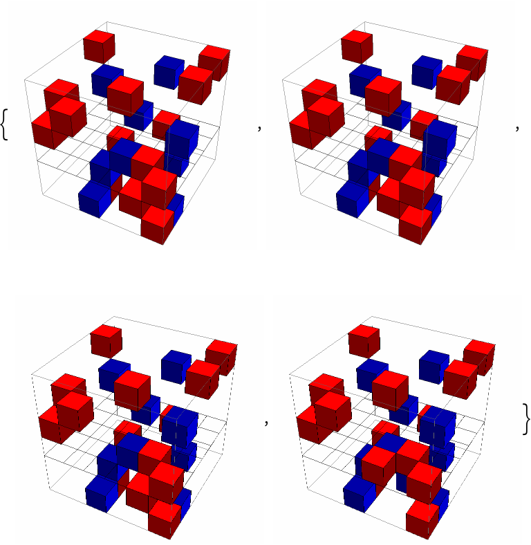 |
Run BBX for 100 steps and 100 more in reverse:
| In[3]:= | ![(* Evaluate this cell to get the example input *) CloudGet["https://www.wolframcloud.com/obj/e8d6e1eb-cc24-4be4-8344-62551d972b4c"]](https://www.wolframcloud.com/obj/resourcesystem/images/68d/68d56c25-e6c9-4c3c-a71d-8c52c9c7de46/6f385d97afdea0c6.png) |
| Out[3]= | 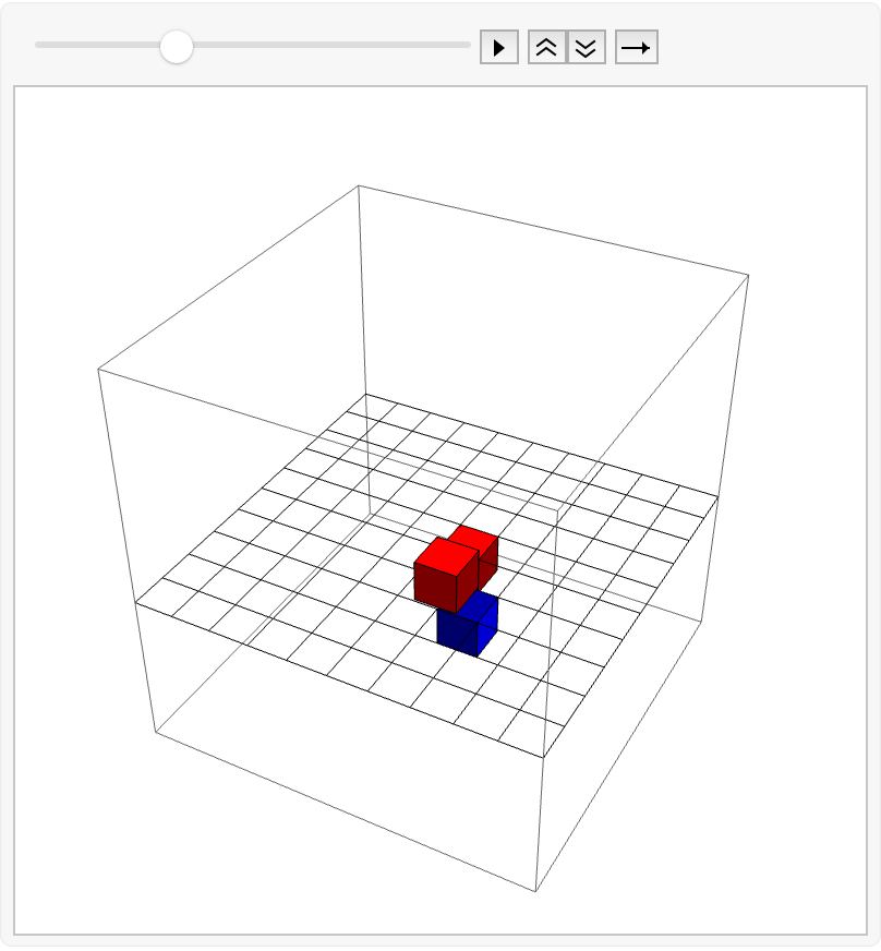 |
Gliders:
| In[4]:= | ![glider1 = SparseArray[{{11, 12, 12} -> 1, {13, 13, 12} -> 1}, {24, 24, 24}];
glider2 = SparseArray[{{12, 11, 14} -> 1, {13, 13, 14} -> 1, {14, 15, 14} -> 1, {15, 17, 14} -> 1}, {24, 24, 24}];
glider3 = SparseArray[{{14, 9, 16} -> 1, {14, 11, 16} -> 1, {13, 11, 16} -> 1, {13, 13, 16} -> 1, {19, 19, 16} -> 1}, {24, 24, 24}];
glider4 = SparseArray[{{15, 9, 18} -> 1, {14, 9, 18} -> 1, {14, 11, 18} -> 1, {13, 11, 18} -> 1, {13, 13, 18} -> 1}, {24, 24, 24}];](https://www.wolframcloud.com/obj/resourcesystem/images/68d/68d56c25-e6c9-4c3c-a71d-8c52c9c7de46/6197ef2ff433ec9b.png) |
| In[5]:= | ![ListAnimate[
ResourceFunction["BusyBoxesAutomaton"]["Visualization"] /@ ResourceFunction["BusyBoxesAutomaton"][glider3, 1000], SaveDefinitions -> True]](https://www.wolframcloud.com/obj/resourcesystem/images/68d/68d56c25-e6c9-4c3c-a71d-8c52c9c7de46/0d0e679b1b8c43a3.png) |
| Out[5]= | 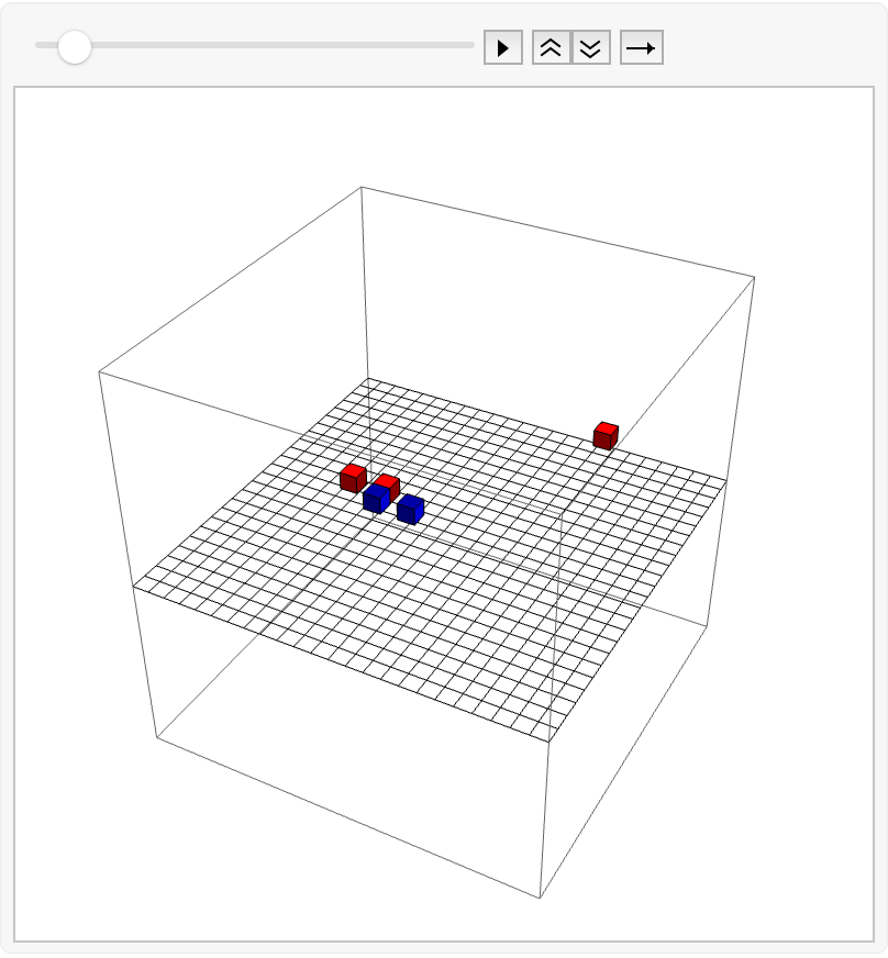 |
| In[6]:= | ![makeBBCircularMotion[n : _Integer?Positive : 3] := Block[{start}, start = {2, -2, 2};
Prepend[
FoldList[Plus, start, Take[Catenate@Table[{{0, 1, -2}, {0, 2, -1}}, Ceiling[n/2]], n]], start + {-2, -1, 0}]
]
makeBBCircularMotion[n : _Integer?Positive : 3, size_Integer] := SparseArray[Thread[makeBBCircularMotion[n] -> 1], ConstantArray[size, 3]]](https://www.wolframcloud.com/obj/resourcesystem/images/68d/68d56c25-e6c9-4c3c-a71d-8c52c9c7de46/5a5ead9e2e302f75.png) |
| In[7]:= | ![Dynamic[If[ListQ[traces], Show[ResourceFunction["BusyBoxesAutomaton"][traces[[-1]], ConstantArray[MinMax[traces] + {-1, 1}, 3], "Visualization", "Grid" -> False], If[ListQ[traces], Graphics3D[{Green, Point /@ Mean /@ traces}], Nothing]], "Run the next cell to start animation"]]](https://www.wolframcloud.com/obj/resourcesystem/images/68d/68d56c25-e6c9-4c3c-a71d-8c52c9c7de46/1c3f2a569072a779.png) |
| Out[7]= | 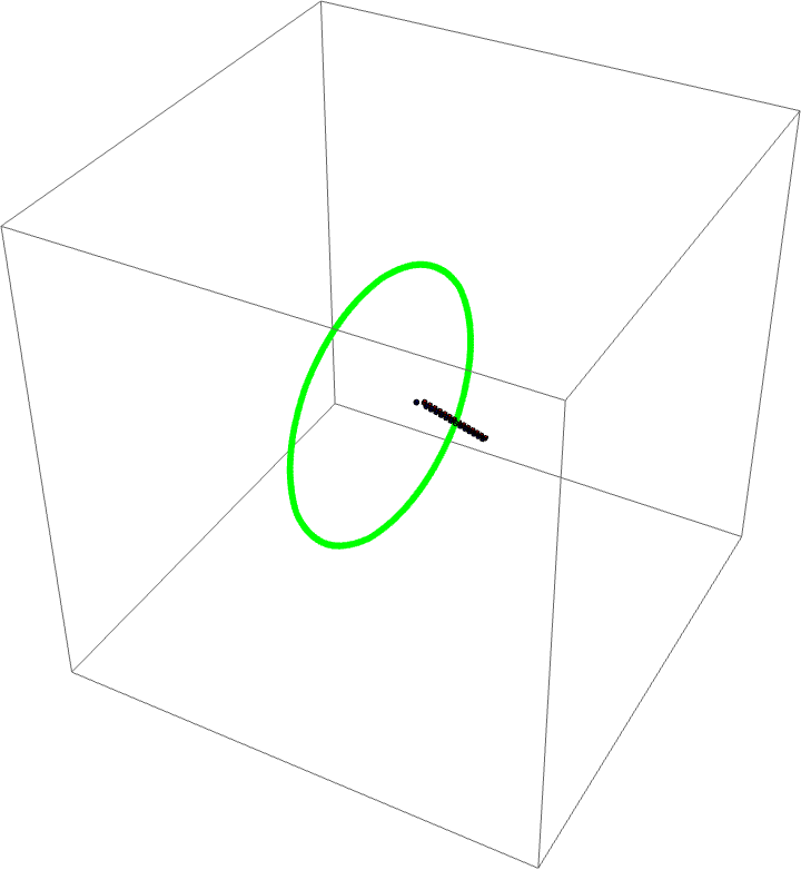 |
Start tracking circular motion:
| In[8]:= | ![n = 28;
traces = {makeBBCircularMotion[n - 2]};
phase = 0;
Until[traces[[1]] === traces[[-1]],
AppendTo[traces, ResourceFunction["BusyBoxesAutomaton"][traces[[-1]], "Step", phase]];
phase = Mod[phase + 1, 6];
]](https://www.wolframcloud.com/obj/resourcesystem/images/68d/68d56c25-e6c9-4c3c-a71d-8c52c9c7de46/10b62e0f649dec79.png) |
Show the circular motion:
| In[9]:= | ![Show[ResourceFunction["BusyBoxesAutomaton"][Catenate[traces], "Visualization", "Grid" -> False], Graphics3D[{Green, Point /@ Mean /@ traces}], PlotRange -> Full]](https://www.wolframcloud.com/obj/resourcesystem/images/68d/68d56c25-e6c9-4c3c-a71d-8c52c9c7de46/632afcc1cc8946d3.png) |
| Out[9]= | 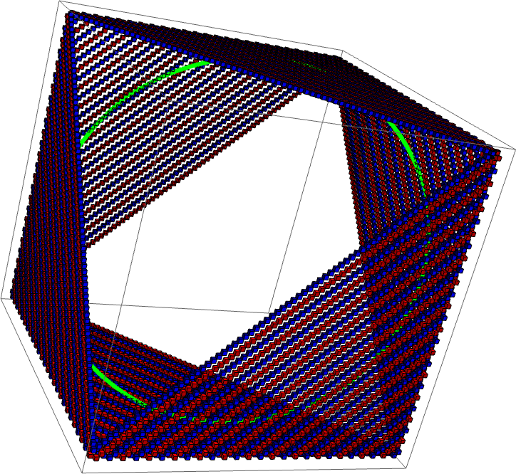 |
Compute box traces for all sizes up-to 100:
| In[10]:= | ![allTraces = Monitor[Table[
NestWhileList[{ResourceFunction["BusyBoxesAutomaton"][#[[1]], "Step", #[[2]]], Mod[#[[2]] + 1, 6]} &, {makeBBCircularMotion[n - 2], 0}, Length[{##}] < n || #1[[1]] != {##}[[-1, 1]] &, All][[;; -2, 1]], {n, 3, 100, 1}], n]; // AbsoluteTiming](https://www.wolframcloud.com/obj/resourcesystem/images/68d/68d56c25-e6c9-4c3c-a71d-8c52c9c7de46/5e991b3be2b0714f.png) |
| Out[10]= |
Plot circularity dependency on the number of boxes measured as standard deviation of average radius for each step:
| In[11]:= | ![ListPlot[
MapIndexed[{#2[[1]] + 2, StandardDeviation[#]/Mean[#] &[
Norm /@ (Mean /@ # - Threaded[Mean[Catenate[#]]])]} &, N@allTraces]]](https://www.wolframcloud.com/obj/resourcesystem/images/68d/68d56c25-e6c9-4c3c-a71d-8c52c9c7de46/75ed6272efc15a48.png) |
| Out[11]= | 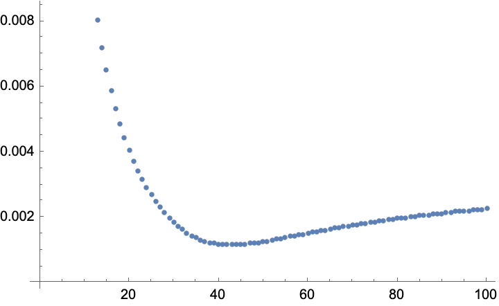 |
Which proves Miller and Fredkin hypothesis wrong of circularity monotonically decreasing to zero. They've only computed this curve up-to 20 boxes, but the minimum is at 43.
Wolfram Language 13.0 (December 2021) or above
This work is licensed under a Creative Commons Attribution 4.0 International License