Wolfram Function Repository
Instant-use add-on functions for the Wolfram Language
Function Repository Resource:
Plot the Bloch sphere
ResourceFunction["BlochSpherePlot"][] plots a labeled Bloch sphere. | |
ResourceFunction["BlochSpherePlot"][{x,y,z}] plots a labeled Bloch sphere together with the Bloch vector {x,y,z}∈ℝ3. | |
ResourceFunction["BlochSpherePlot"][{{x1,y1,z1},…,{xn,yn,zn}}] shows multiple vectors in ℝ3. | |
ResourceFunction["BlochSpherePlot"][{α,β}] plots a labeled Bloch sphere together with the Bloch vector of the quantum state {α,β}∈ℂ2. | |
ResourceFunction["BlochSpherePlot"][{{α1,β1},…,{αn,βn}}] shows multiple quantum states in ℂ2. | |
ResourceFunction["BlochSpherePlot"][ρ] plots a labeled Bloch sphere together with the Bloch vector of the quantum density matrix ρ∈ℂ2⊗ℂ2. | |
ResourceFunction["BlochSpherePlot"][{ρ1,…,ρn}] plots a labeled Bloch sphere together with Bloch vectors of quantum density matrices ρi∈ℂ2⊗ℂ2. |
| "NumberOfGreatCircles" | 2 | number of great circles (also called parallels) whose centers are the same as the sphere’s center |
| "ShowGreatCircles" | True | if False, the great circles will not be shown |
| "NumberOfSmallCircles" | 1 | number of small circles (also called meridians) whose centers are along z-axis |
| "ShowSmallCircles" | True | if False, the small circles will not be shown |
| "Labels" | Automatic | labels of axes, based on common kets for the eigenstates of Pauli operators. If it is set as "Optics" the common optics labels as will be used. |
| "LabelPositions" | Automatic | positions of labels in the Bloch sphere |
| "ShowLabels" | True | if False, axes labels will not be shown |
| "ShowAxes" | True | if False, the customized axes will not be shown |
| "ForceStateVector" | False | if True, the input is interpreted as state vector |
Plot the Bloch sphere:
| In[1]:= |
| Out[1]= |  |
Plot the Bloch sphere for a Bloch vector:
| In[2]:= |
| Out[2]= | 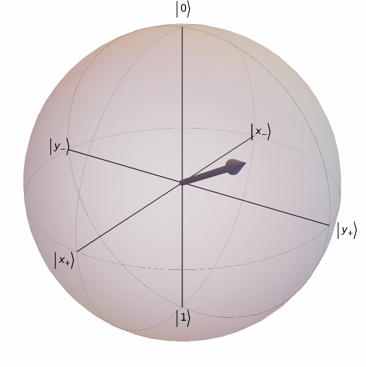 |
Plot the Bloch sphere for some random Bloch vectors:
| In[3]:= |
| Out[3]= | 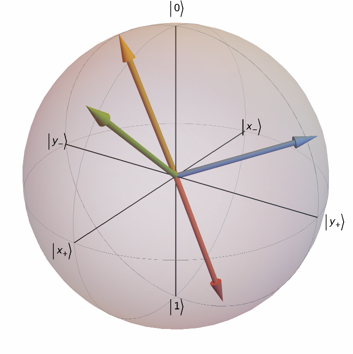 |
Plot the Bloch sphere for the quantum state {Cos[π/6],-ⅇⅈπ/4Sin[π/6]}:
| In[4]:= |
| Out[4]= | 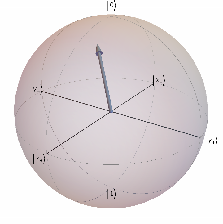 |
Plot the Bloch sphere for a list of random pure quantum states:
| In[5]:= |
| Out[5]= | 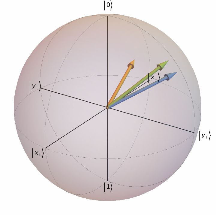 |
Plot the Bloch sphere for a random density matrix:
| In[6]:= |
| Out[6]= | 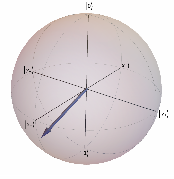 |
Plot the Bloch sphere for a list of random density matrices:
| In[7]:= | ![ResourceFunction[
"BlochSpherePlot", ResourceSystemBase -> "https://www.wolframcloud.com/obj/resourcesystem/api/1.0"][
Table[1/2 (IdentityMatrix[2] + RandomPoint[Ball[]] . Table[PauliMatrix[j], {j, 3}]), 5]]](https://www.wolframcloud.com/obj/resourcesystem/images/fcb/fcb3b840-6ae5-4883-a256-1573cc958ffc/0eaa83de626de345.png) |
| Out[7]= | 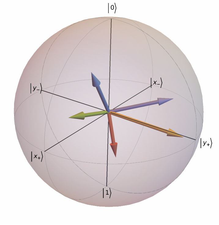 |
Add more great circles (also called parallels):
| In[8]:= |
| Out[8]= | 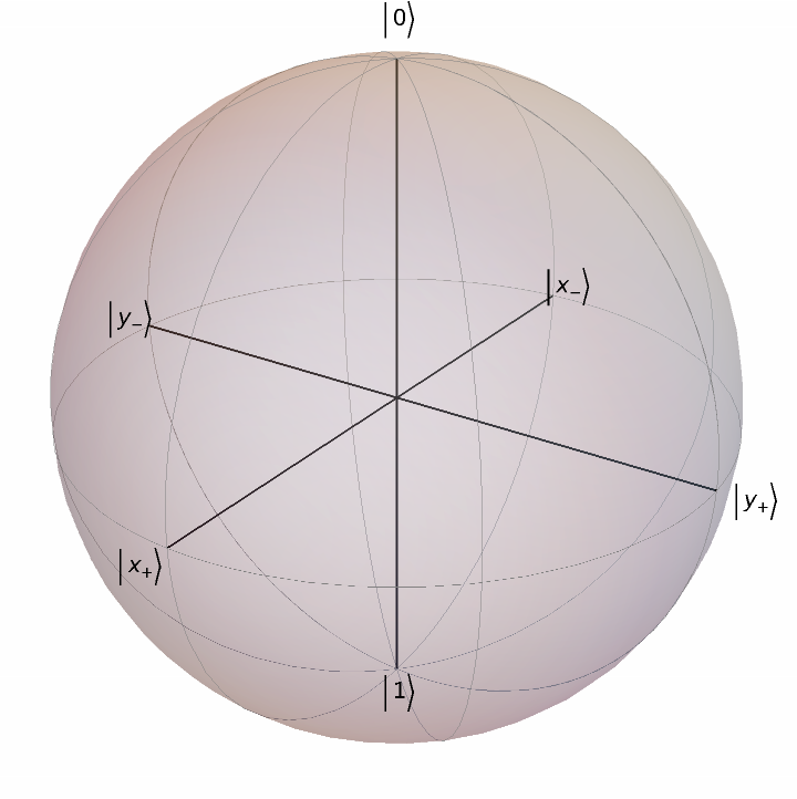 |
Turn off great circles:
| In[9]:= |
| Out[9]= | 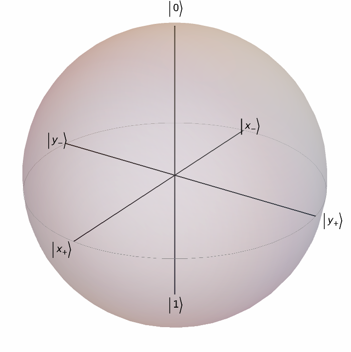 |
Add more small circles (also called meridians):
| In[10]:= |
| Out[10]= | 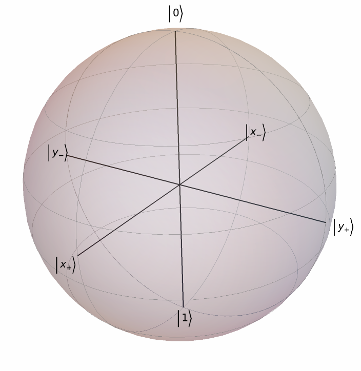 |
Turn off small circles:
| In[11]:= |
| Out[11]= |  |
Show common labels in optics:
| In[12]:= |
| Out[12]= |  |
Show customized labels:
| In[13]:= |
| Out[13]= |  |
Customize labels positions:
| In[14]:= |
| Out[14]= | 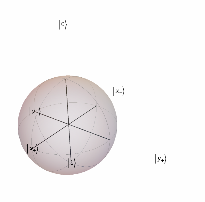 |
Turn off labels:
| In[15]:= |
| Out[15]= | 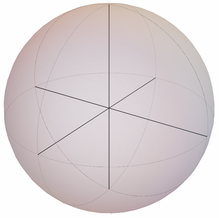 |
Do not show axes:
| In[16]:= |
| Out[16]= | 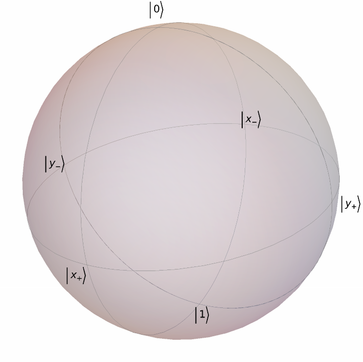 |
Force the state vector interpretation:
| In[17]:= |
| Out[17]= |  |
Given an initial quantum state, plot the state after bit-flip and phase-flip errors:
| In[18]:= | ![\[Psi]0 = {Cos[\[Pi]/8], Exp[I \[Pi]/3] Sin[\[Pi]/8]};
ResourceFunction[
"BlochSpherePlot", ResourceSystemBase -> "https://www.wolframcloud.com/obj/resourcesystem/api/1.0"][{\[Psi]0, PauliMatrix[3] . \[Psi]0, PauliMatrix[2] . \[Psi]0}]](https://www.wolframcloud.com/obj/resourcesystem/images/fcb/fcb3b840-6ae5-4883-a256-1573cc958ffc/5c82393524077ba3.png) |
| Out[19]= | 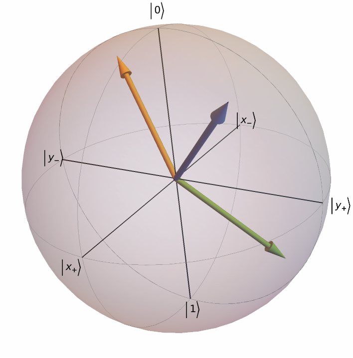 |
Given the initial Bloch vector {0,0,1}, plot the state rotation around y-axis by the angles {π/6,π/3,2π/3}:
| In[20]:= |
| Out[20]= | 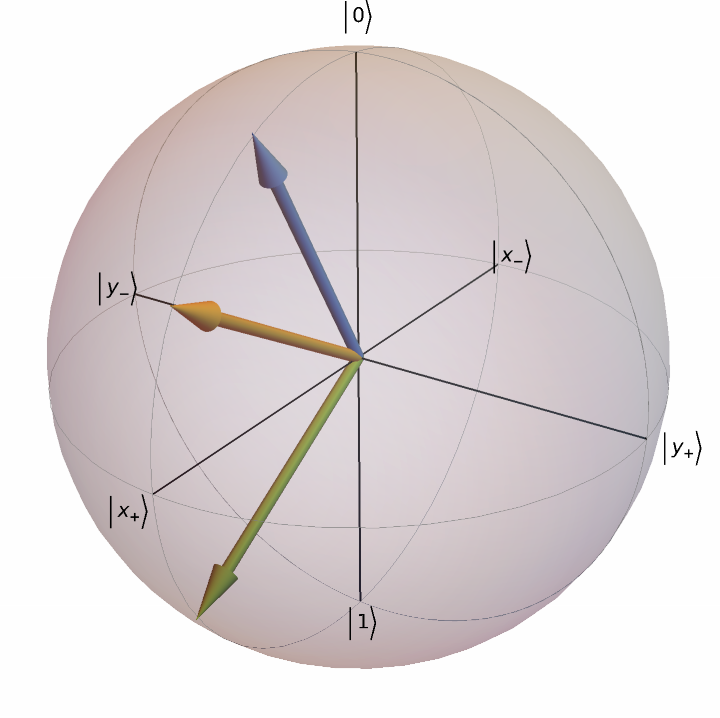 |
The input should be a list of vectors as {x,y,z}ϵ ℝ2, or state vectors {α,β}∈ ℂ2 or density matrices:
| In[21]:= |
| Out[21]= |
If the states are out of the Bloch sphere, it means they are not physically accessible states:
| In[22]:= |
| Out[22]= | 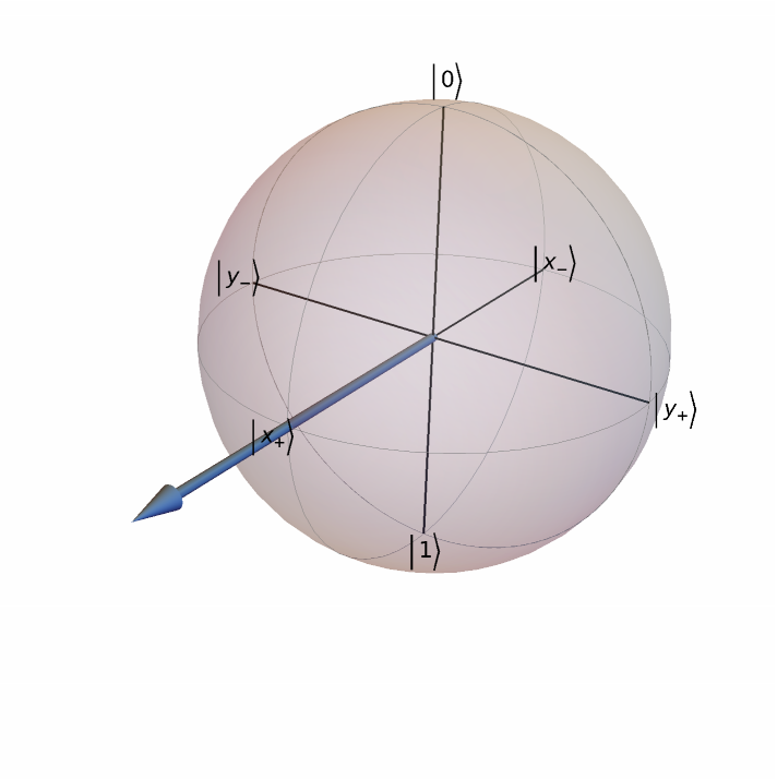 |
A list of two state vectors can be also interpreted as a density matrix, such as {{1,0},{0,1}}:
| In[23]:= |
| Out[23]= |  |
Force the state vector interpretation:
| In[24]:= |
| Out[24]= | 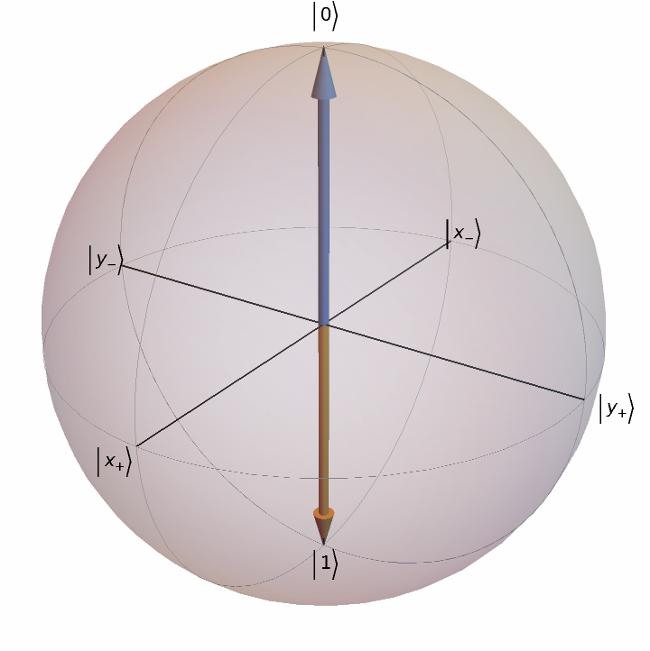 |
Plot a generic pure state as {Cos[θ/2],ⅇⅈ ϕSin[θ/2]}:
| In[25]:= | ![Manipulate[
ResourceFunction[
"BlochSpherePlot", ResourceSystemBase -> "https://www.wolframcloud.com/obj/resourcesystem/api/1.0"][{Cos[\[Theta]/2], Sin[\[Theta]/2] Exp[I \[Phi]]}], {\[Theta], 0, \[Pi]}, {\[Phi], 0, 2 \[Pi]}, SaveDefinitions -> True]](https://www.wolframcloud.com/obj/resourcesystem/images/fcb/fcb3b840-6ae5-4883-a256-1573cc958ffc/6e9715d09fc33ba9.png) |
| Out[25]= |  |
Wolfram Language 13.0 (December 2021) or above
This work is licensed under a Creative Commons Attribution 4.0 International License

