Wolfram Function Repository
Instant-use add-on functions for the Wolfram Language
Function Repository Resource:
Solve an orthogonal polynomial Vandermonde linear system
ResourceFunction["OrthogonalPolynomialVandermondeSolve"][poly,{a1,a2,…},{b1,b2,…}] solves the primal Vandermonde problem V.x==b, where V(a1,a2,…) is the orthogonal polynomial Vandermonde matrix with respect to the basis represented by poly. |
| "ChebyshevFirst" | Chebyshev polynomial of the first kind ChebyshevT[i,x] |
| "ChebyshevSecond" | Chebyshev polynomial of the second kind ChebyshevU[i,x] |
| "Hermite" | Hermite polynomial HermiteH[i,x] |
| "Laguerre" | Laguerre polynomial LaguerreL[i,x] |
| "Legendre" | Legendre polynomial LegendreP[i,x] |
| {"Gebenbauer",m} | Gegenbauer polynomial GegenbauerC[i,m,x] |
| {"Laguerre",a} | associated Laguerre polynomial LaguerreL[i,a,x] |
| {"Jacobi",a,b} | Jacobi polynomial JacobiP[i,a,b,x] |
Solve a Chebyshev–Vandermonde system:
| In[1]:= |
|
| Out[1]= |
|
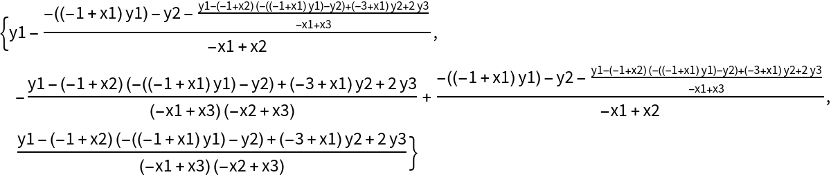
Solve a Jacobi–Vandermonde system with symbolic parameters and vectors:
| In[2]:= |
|
| Out[2]= |
|
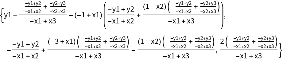
An equivalent specification:
| In[3]:= |
|
| Out[3]= |
|
Solve a Hermite–Vandermonde system with numeric vectors:
| In[4]:= |
|
| Out[4]= |
|
Get the Legendre series coefficients of an interpolating polynomial:
| In[9]:= |
![pts = {{0., 0.}, {0.1, 0.3}, {0.5, 0.6}, {1., -0.2}, {2., 3.}};
cc = ResourceFunction["OrthogonalPolynomialVandermondeSolve"][
"Legendre", pts[[All, 1]], pts[[All, 2]], "Transpose" -> True]](https://www.wolframcloud.com/obj/resourcesystem/images/7d5/7d5419cf-5180-4b7e-9479-62a412a81910/057010fb62418379.png)
|
| Out[10]= |
|
Use the resource function OrthogonalPolynomialSum to get the corresponding orthogonal polynomial series, and compare with the result of InterpolatingPolynomial:
| In[11]:= |
|
| Out[11]= |
|
OrthogonalPolynomialVandermondeSolve is more efficient than using LinearSolve on an orthogonal polynomial Vandermonde system:
| In[12]:= |
|
| In[13]:= |
|
| Out[13]= |
|
| In[14]:= |
![AbsoluteTiming[
c2 = LinearSolve[
ResourceFunction["OrthogonalPolynomialVandermondeMatrix"][
"Hermite", N[xr]], N[yr]];]](https://www.wolframcloud.com/obj/resourcesystem/images/7d5/7d5419cf-5180-4b7e-9479-62a412a81910/06346f15157f9051.png)
|
| Out[14]= |
|
The result of OrthogonalPolynomialVandermondeSolve is also often more accurate:
| In[15]:= |
|
| In[16]:= |
|
| Out[16]= |
|
| In[17]:= |
|
| Out[17]= |
|
This work is licensed under a Creative Commons Attribution 4.0 International License
![% == LinearSolve[
Transpose@
ResourceFunction["OrthogonalPolynomialVandermondeMatrix"][
"Laguerre", {x1, x2, x3}], {y1, y2, y3}] // Simplify](https://www.wolframcloud.com/obj/resourcesystem/images/7d5/7d5419cf-5180-4b7e-9479-62a412a81910/2ae3b945639741d9.png)
