Basic Examples (5)
Identify the exact gaps in a non-convex subset:
A convex set has no defect:
The defect size quantifies "how far" from convex:
Non-contiguous parent set:
The empty set has no defect:
Scope (4)
Works with rational elements:
Works with strings under canonical (lexicographic) order:
Works with symbolic heads that have a canonical ordering:
A singleton always has an empty defect:
Options (2)
ConvexDefect supports a "ComparisonFunction" option to specify a custom ordering. Under such an ordering, the defect reflects the gaps with respect to the induced order:
Under the default LessEqual, the same call gives a different defect because the canonical order is lexicographic, not length-based:
Applications (3)
Identify missing sensor readings in an active measurement range:
Find which days are missing from a schedule within its active range:
Detect missing entries in a sorted database key range:
Properties and Relations (5)
OrderConvexQ returns True if and only if the defect is empty:
The defect size equals the number of elements in the interval Interval[MinMax[subset]] relative to parent set that are not in the subset:
The interval induced by a subset decomposes into the subset and its defect:
A subset containing all elements of its induced interval has empty defect:
Monotonicity. If , then :
Possible Issues (1)
Requires a finite totally ordered parent set; elements must admit comparison via LessEqual or a user-defined ordering. Does not verify . If subset contains elements absent from parent set, the defect is computed relative to the closure filtered from parent set. If subset contains elements not in parent set, the defect only reports gaps from parent set:
The elements 2 and 8 act as bounds but are not themselves in parent set, so the entire closure interval from parent set appears as defect.
Neat Examples (3)
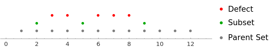
Visualize the convex defect of a subset on a number line. Grey marks the parent set, green the subset, red the defect (the missing elements):
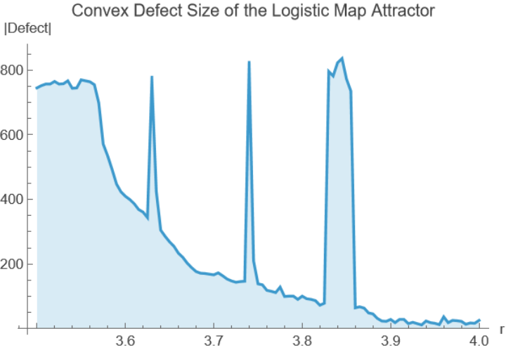
Plot how the defect size of the logistic map orbit varies with the parameter . The defect measures the number of grid points within the convex hull of the attractor that are not visited by the orbit at the chosen resolution, providing a discrete fingerprint of its Cantor-like fractal structure:
The spikes correspond to periodic windows where the orbit collapses to a finite cycle, leaving a large convex hull mostly empty. Outside these windows, the defect decreases as the chaotic attractor becomes increasingly dense in the interval. At , the defect approaches zero, the orbit densely fills , leaving no gaps at the chosen discretization scale.
Compare the defect structure at two contrasting parameter values, one inside a periodic window (, period-3) and one fully chaotic ():
At , the system lies within a period-3 window of the logistic map. The orbit settles onto a 3-cycle whose three limit points occupy a negligible portion of the convex hull, leaving 796 out of roughly 800 grid points as defect - an essentially hollow interval. This provides a discrete manifestation of the fact that stable periodic orbits have zero Lebesgue measure.
At , the situation is subtler. The map is topologically conjugate to the tent map via the Ulam–von Neumann substitution , and its invariant measure is the arcsine distribution
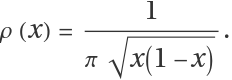
The density diverges at the endpoints and attains its minimum at , so the orbit samples the interval least frequently near its center. The observed defect of 1 at resolution 0.001 reflects this: even after iterations, the region of minimal invariant density may still contain a grid point not yet visited by the orbit. In the , limit the defect vanishes, consistent with the ergodicity of the fully chaotic regime.
![ResourceFunction["ConvexDefect"][{"ab", "abcde"},
{"a", "ab", "xyz", "test", "abcde", "longer"},
"ComparisonFunction" -> Function[LessEqual[StringLength[#], StringLength @ #2]]
]](https://www.wolframcloud.com/obj/resourcesystem/images/670/67000b8e-4db2-4302-96b0-0304a129695f/1c4dff124f97f7fe.png)
![ResourceFunction["ConvexDefect"][{"ab", "abcde"},
{"a", "ab", "xyz", "test", "abcde", "longer"}
]](https://www.wolframcloud.com/obj/resourcesystem/images/670/67000b8e-4db2-4302-96b0-0304a129695f/028ac81f074c6725.png)
![With[
{
allDays = Range[1, 31],
scheduled = {5, 6, 7, 8, 10, 11, 12, 13, 14, 15}
},
ResourceFunction["ConvexDefect"][scheduled, allDays]
]](https://www.wolframcloud.com/obj/resourcesystem/images/670/67000b8e-4db2-4302-96b0-0304a129695f/7bafd7a2de58cd63.png)
![With[{s = {2, 3, 5}, p = Range @ 10},
SameQ[ResourceFunction["OrderConvexQ"][s, p],
SameQ[ResourceFunction["ConvexDefect"][s, p], {}]
]
]](https://www.wolframcloud.com/obj/resourcesystem/images/670/67000b8e-4db2-4302-96b0-0304a129695f/418839521a985e4e.png)
![With[{s = {1, 5, 9}, p = Range @ 10},
Equal[Length @ ResourceFunction["ConvexDefect"][s, p],
Length[Select[p, LessEqual[Min[s], #, Max @ s] &]] - Length[s]
]
]](https://www.wolframcloud.com/obj/resourcesystem/images/670/67000b8e-4db2-4302-96b0-0304a129695f/0d89922950695dd0.png)
![With[{s = {1, 3, 7}, p = Range @ 10},
SameQ[Sort[Select[p, LessEqual[Min @ s, #, Max @ s] &]],
Sort @ Join[s, ResourceFunction["ConvexDefect"][s, p]]
]
]](https://www.wolframcloud.com/obj/resourcesystem/images/670/67000b8e-4db2-4302-96b0-0304a129695f/3f8ba344eead7f27.png)
![With[{s = {2, 8}, p = Range @ 10},
ResourceFunction["ConvexDefect"][
Select[p, LessEqual[Min @ s, #, Max @ s] &], p]
]](https://www.wolframcloud.com/obj/resourcesystem/images/670/67000b8e-4db2-4302-96b0-0304a129695f/0fcba2849d20a1f1.png)
![With[
{
p = Range @ 10,
a = {2, 8},
b = {2, 5, 8}
},
SubsetQ[ResourceFunction["ConvexDefect"][a, p], ResourceFunction["ConvexDefect"][b, p]]
]](https://www.wolframcloud.com/obj/resourcesystem/images/670/67000b8e-4db2-4302-96b0-0304a129695f/263672cb2a4124e4.png)
![With[{s = {2, 5, 9}, p = Range @ 12},
NumberLinePlot[{p, s, ResourceFunction["ConvexDefect"][s, p]},
PlotStyle -> {Gray, Darker[Green], Red},
PlotLegends -> {"Parent Set", "Subset", "Defect"},
Spacings -> 0.5
]
]](https://www.wolframcloud.com/obj/resourcesystem/images/670/67000b8e-4db2-4302-96b0-0304a129695f/67768c404266f47e.png)
![ListLinePlot[
Table[
Module[{grid, orbit, disc},
grid = Range[0., 1., 0.001];
orbit = NestList[Function[r * # * (1 - #)], 0.1, 5000];
disc = DeleteDuplicates @ Round[orbit, 0.001];
{r, Length @ ResourceFunction["ConvexDefect"][disc, grid]}
],
{r, 3.5, 4., 0.005}
],
AxesLabel -> {"r", "|Defect|"},
PlotLabel -> "Convex Defect Size of the Logistic Map Attractor", Filling -> Bottom, PlotRange -> All
]](https://www.wolframcloud.com/obj/resourcesystem/images/670/67000b8e-4db2-4302-96b0-0304a129695f/78391c133c9c1f28.png)
![With[{res = 0.001},
Module[{grid, f},
grid = Range[0., 1., res];
f[
Pattern[r,
Blank[]]] := Module[
{disc},
disc = DeleteDuplicates[
Round[NestList[Function[r * # * (1 - #)], 0.1, 10000], res]
];
ResourceFunction["ConvexDefect"][disc, grid]
];
Column @ {
Row @ {"r = 3.83: |Defect| = ", Length @ f @ 3.83},
Row @ {"r = 4.00: |Defect| = ", Length @ f @ 4.}
}
]
]](https://www.wolframcloud.com/obj/resourcesystem/images/670/67000b8e-4db2-4302-96b0-0304a129695f/7ceca66d1e6b8526.png)