Wolfram Function Repository
Instant-use add-on functions for the Wolfram Language
Function Repository Resource:
Compute the discrete Hilbert transform of a list
| ResourceFunction["DiscreteHilbertTransform"][list] computes the discrete Hilbert transform of a list of real numbers. | 
Compute a discrete Hilbert transform:
| In[1]:= | ![ResourceFunction["DiscreteHilbertTransform"][{1, 1, 2, 2, 1, 1, 0, 0}]](https://www.wolframcloud.com/obj/resourcesystem/images/634/634472b1-61f8-47d9-853f-ac67378e9810/3b55f8de6615d335.png) | 
| Out[1]= |  | 
x is a list of real values:
| In[2]:= |  | 
Compute the Hilbert transform with machine arithmetic:
| In[3]:= | ![ResourceFunction["DiscreteHilbertTransform"][x]](https://www.wolframcloud.com/obj/resourcesystem/images/634/634472b1-61f8-47d9-853f-ac67378e9810/4214a010f8f50109.png) | 
| Out[3]= |  | 
Compute using 24-digit precision arithmetic:
| In[4]:= | ![ResourceFunction["DiscreteHilbertTransform"][N[x, 24]]](https://www.wolframcloud.com/obj/resourcesystem/images/634/634472b1-61f8-47d9-853f-ac67378e9810/413d40f7c0ce76ef.png) | 
| Out[4]= |  | 
Compute a 2D Hilbert transform:
| In[5]:= | ![ResourceFunction["DiscreteHilbertTransform"][
 RandomReal[{-1, 1}, {3, 6}]]](https://www.wolframcloud.com/obj/resourcesystem/images/634/634472b1-61f8-47d9-853f-ac67378e9810/7dcdf0af975c87a7.png) | 
| Out[5]= |  | 
Generate a sequence composed of two sinusoids with some noise:
| In[6]:= | ![data = Cos[203*2 \[Pi]*Range[0, 1, 0.001]] + Sin[721*2 \[Pi]*Range[0, 1, 0.001]] + RandomVariate[NormalDistribution[0, 0.001], 1001];](https://www.wolframcloud.com/obj/resourcesystem/images/634/634472b1-61f8-47d9-853f-ac67378e9810/4d6544c50813811c.png) | 
Compute the discrete Hilbert transform:
| In[7]:= | ![Short[ht = ResourceFunction["DiscreteHilbertTransform"][data]]](https://www.wolframcloud.com/obj/resourcesystem/images/634/634472b1-61f8-47d9-853f-ac67378e9810/03421f86be4d97b0.png) | 
| Out[7]= |  | 
Visualize the "analytic signal" by separately plotting its real part (the original data) and imaginary part (the Hilbert transform):
| In[8]:= | ![ListLinePlot[{data, ht}, DataRange -> {0, 1}, Joined -> True, PlotLegends -> {"original data", "Hilbert transform"}, PlotRange -> {{0.01, 0.07}, Automatic}]](https://www.wolframcloud.com/obj/resourcesystem/images/634/634472b1-61f8-47d9-853f-ac67378e9810/0e069ce57484589b.png) | 
| Out[8]= |  | 
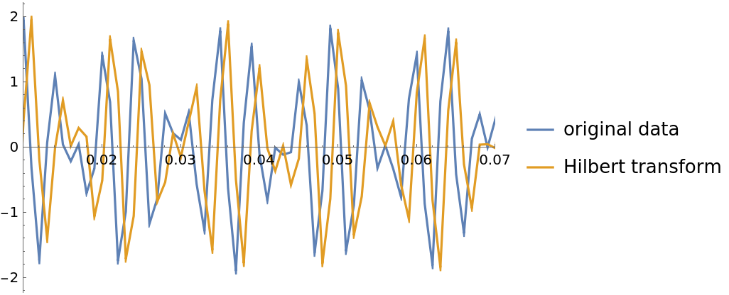
Use the resource function WelchSpectralEstimate to compare the power spectral densities of the original sequence and the "analytic signal":
| In[9]:= | ![ListLogLogPlot[{ResourceFunction["WelchSpectralEstimate"][data, 100.0,
    "OneSided" -> False], ResourceFunction["WelchSpectralEstimate"][data + I ht, 100.0, "OneSided" -> False]}, Joined -> True, PlotLegends -> {"original PSD", "Hilbert PSD"}]](https://www.wolframcloud.com/obj/resourcesystem/images/634/634472b1-61f8-47d9-853f-ac67378e9810/6c9aee4c6c1599ff.png) | 
| Out[9]= |  | 
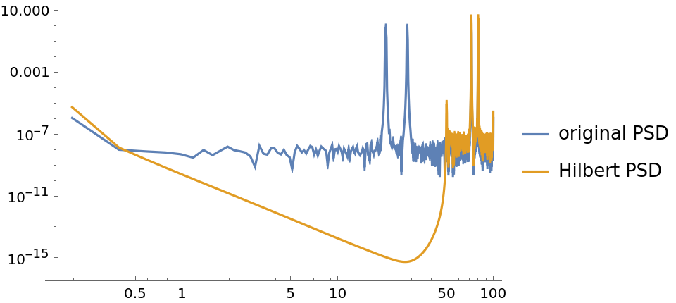
A vector of real values:
| In[10]:= |  | 
Compute its Hilbert transform:
| In[11]:= | ![ht = ResourceFunction["DiscreteHilbertTransform"][x]](https://www.wolframcloud.com/obj/resourcesystem/images/634/634472b1-61f8-47d9-853f-ac67378e9810/44ab0917c460b21d.png) | 
| Out[11]= |  | 
The dot product of the Hilbert transform with the original vector is zero:
| In[12]:= |  | 
| Out[12]= |  | 
Compute the discrete Hilbert transform of a vector by multiplying it with the Hilbert transform matrix:
| In[13]:= | ![u = N[{1, 2, 3, 4, 5, 6, 7}];
n = Length[u];](https://www.wolframcloud.com/obj/resourcesystem/images/634/634472b1-61f8-47d9-853f-ac67378e9810/09d776c32283a2a1.png) | 
| In[14]:= | ![AbsoluteTiming[
 v1 = ResourceFunction["DiscreteHilbertTransformMatrix"][n] . u]](https://www.wolframcloud.com/obj/resourcesystem/images/634/634472b1-61f8-47d9-853f-ac67378e9810/3b260f85d25ae416.png) | 
| Out[14]= |  | 
DiscreteHilbertTransform is faster:
| In[15]:= | ![AbsoluteTiming[v2 = ResourceFunction["DiscreteHilbertTransform"][u]]](https://www.wolframcloud.com/obj/resourcesystem/images/634/634472b1-61f8-47d9-853f-ac67378e9810/3f17f212e85125bd.png) | 
| Out[15]= |  | 
| In[16]:= | ![Chop[v1 - v2]](https://www.wolframcloud.com/obj/resourcesystem/images/634/634472b1-61f8-47d9-853f-ac67378e9810/007686af23cf1367.png) | 
| Out[16]= |  | 
An even-length sequence:
| In[17]:= | ![v = RandomVariate[NormalDistribution[], 8]](https://www.wolframcloud.com/obj/resourcesystem/images/634/634472b1-61f8-47d9-853f-ac67378e9810/1abc2b58adb6f3a3.png) | 
| Out[17]= |  | 
Use the discrete Hartley transform to compute the discrete Hilbert transform:
| In[18]:= | ![ResourceFunction["DiscreteHartleyTransform"][
 RotateRight[
   Reverse[ResourceFunction["DiscreteHartleyTransform"][v]]] Join[{0},
    ConstantArray[1, Length[v]/2 - 1], {0}, ConstantArray[-1, Length[v]/2 - 1]]]](https://www.wolframcloud.com/obj/resourcesystem/images/634/634472b1-61f8-47d9-853f-ac67378e9810/78cfffe8a9463090.png) | 
| Out[18]= |  | 
Compare with the result of DiscreteHilbertTransform:
| In[19]:= | ![ResourceFunction["DiscreteHilbertTransform"][v]](https://www.wolframcloud.com/obj/resourcesystem/images/634/634472b1-61f8-47d9-853f-ac67378e9810/019bdc10e47fbd8e.png) | 
| Out[19]= |  | 
This work is licensed under a Creative Commons Attribution 4.0 International License