Basic Examples (2)
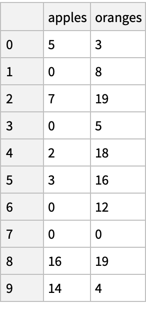
Create a dataset of the purchases of some individuals:
Transfer the dataset from Python:
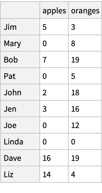
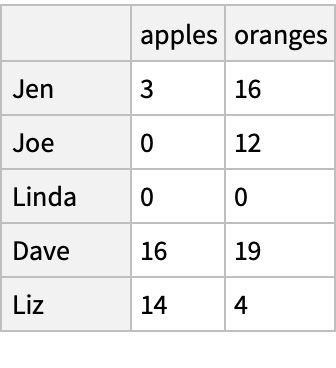
Attach customer names to the purchases, using the names as "index" (labels of the rows):
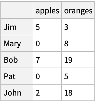
Get several rows from the beginning and the end of the dataset:
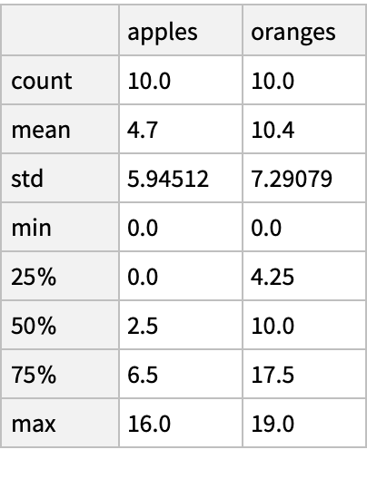
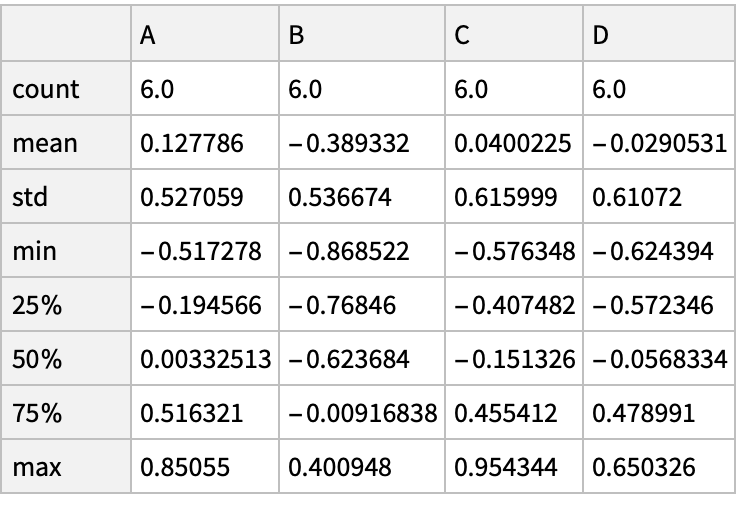
Generate descriptive statistics of the purchases:
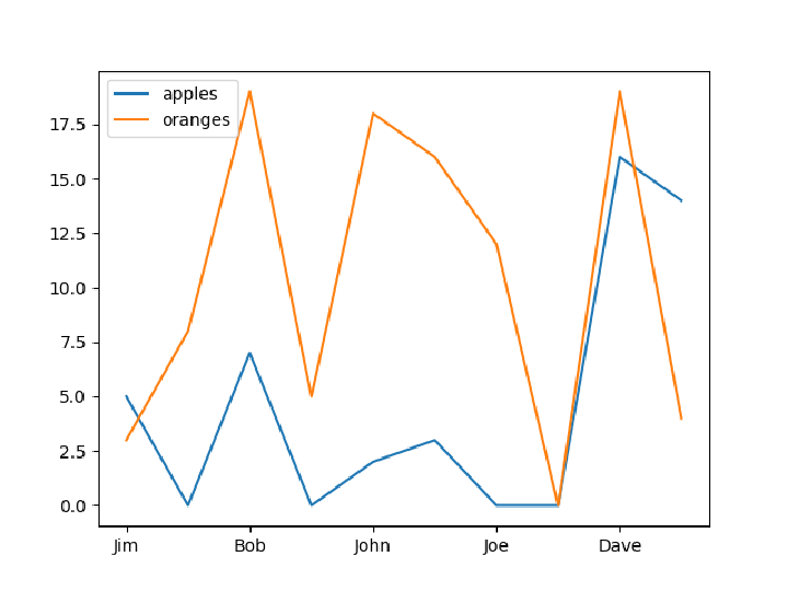
Create and display a plot of the purchases:
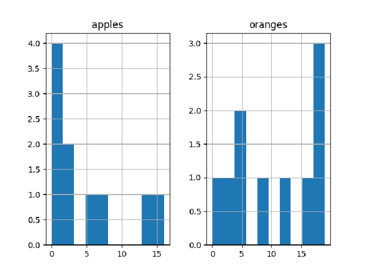
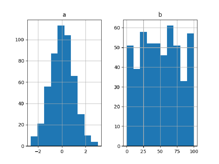
Histograms of the purchases:
Close the Python session to clean up:
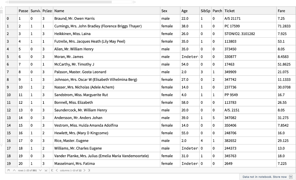
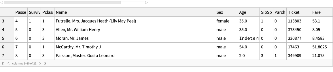
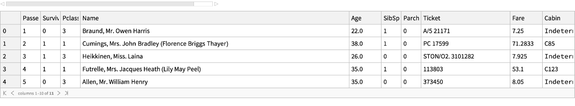
Load the Titanic disaster data:
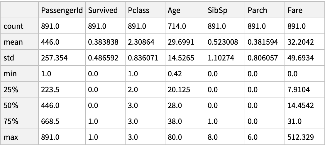
The descriptive statistics of the dataset:
The average fare paid:
The median age and fare of the passengers:
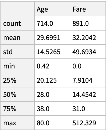
Descriptive statistics of the specified columns:
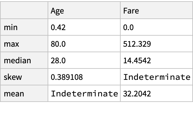
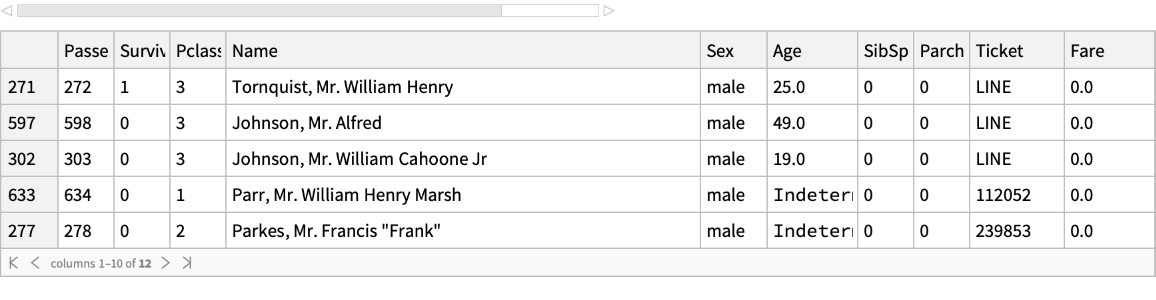
Use the specific aggregating statistics for given columns instead of the predefined statistics:
Find the number of male and female passengers:
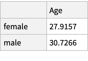
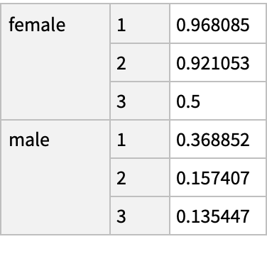
The average age for male versus female passengers:
Count the number of unique values in all the columns:
Or in a specific column:
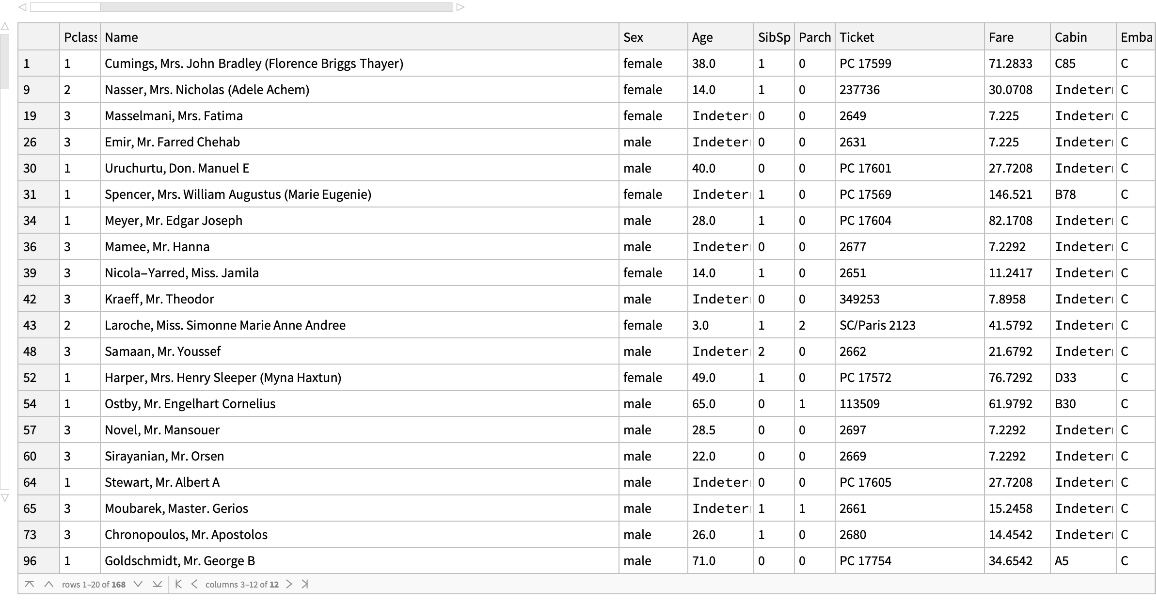
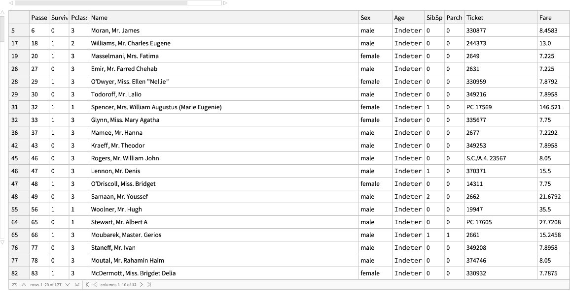
Pick passengers who embarked at the port "C" (Cherbourg):
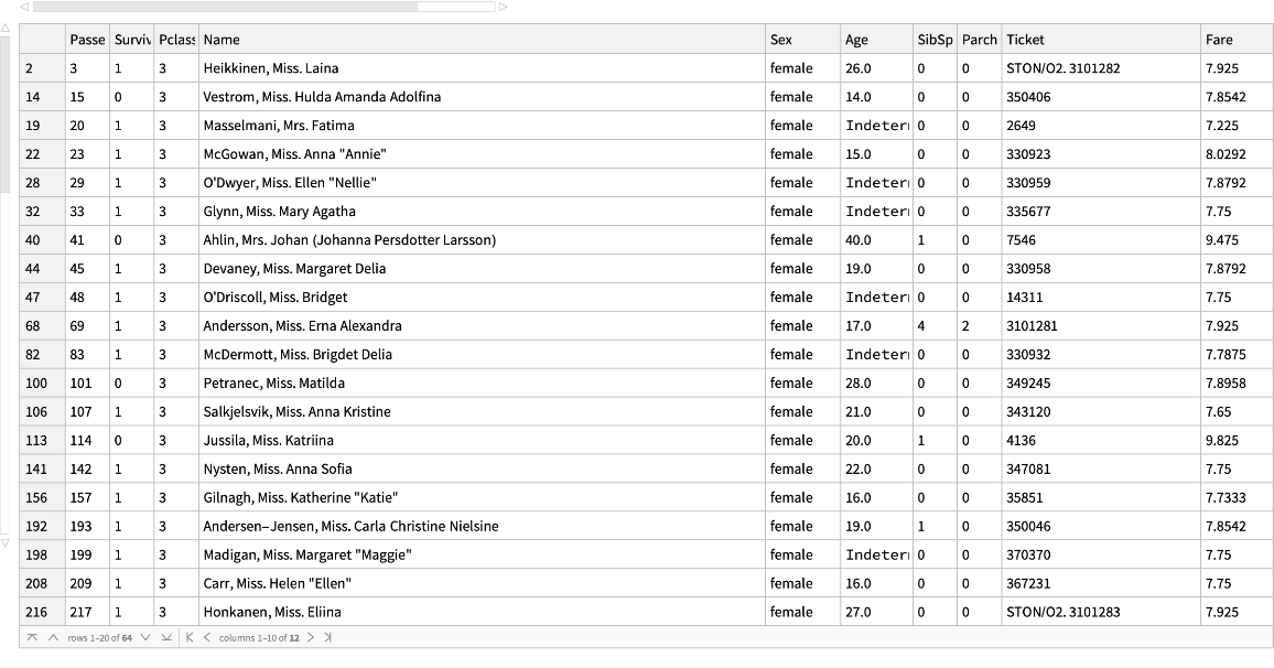
Female passengers, whose fare was less than $10:
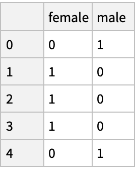
Find the correlation between the sex and survival by replacing string values in the "Sex" column with numbers using the String method "GetDummies" ("women first"):
Summarize the survival rate by sex and cabin class using a spreadsheet-like pivot table (better survival rate for women and in the first class):
Find the missing values in the "Age" column:
Statistics is calculated despite missing values:
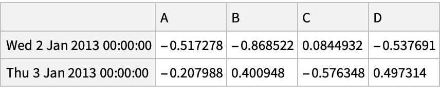
Drop the first few rows by giving the index values as labels and specifying "Axis"→0 for a row-wise operation:
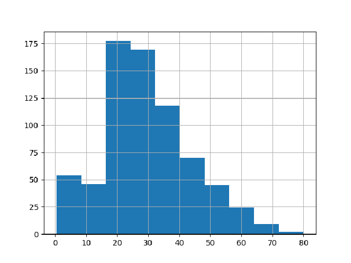
Prepare and show a histogram of age values:
Drop the specified column:
Create a copy of the object:
Drop the "Sex" column in the object in-place:
Sort the data by values of the specified column:
Prepare and show stacked filled plots of the numeric columns:
Clean up the Python session:
Scope (125)
Object creation (2)
Create a Series object from a list of values, letting pandas use a default integer index:
Create a new panda object:
Create a date-time index array of six values by specifying the starting date in the form "yyyy-mm-dd":
Alternatively, specify the starting date without dashes:
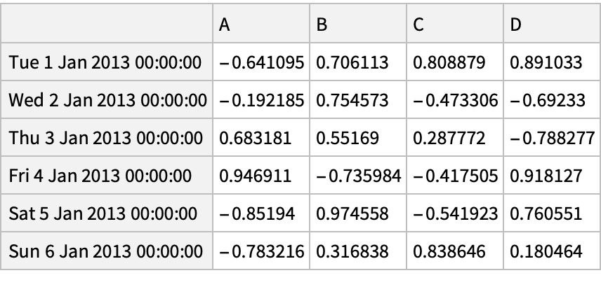
Construct a "DataFrame" object from the array of dates with labeled columns:
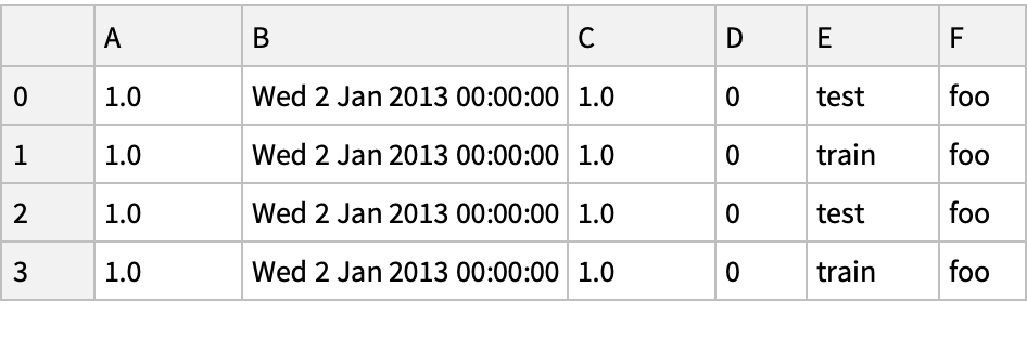
Create a "DataFrame" from an association of objects that can be converted into a "Series"-like structure:
Viewing data (16)
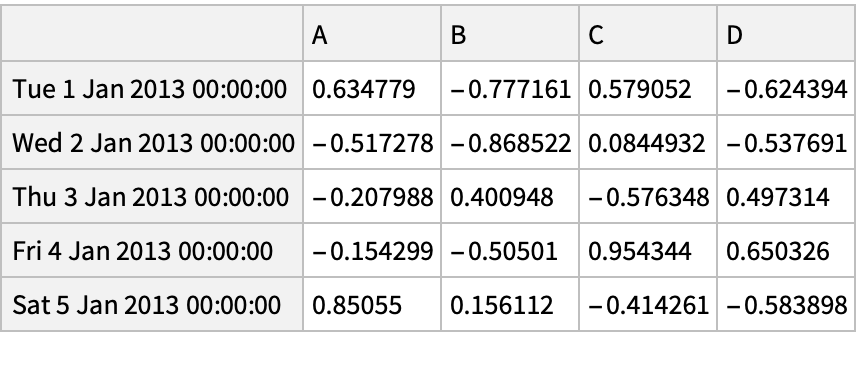
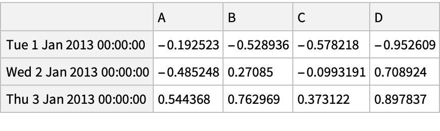
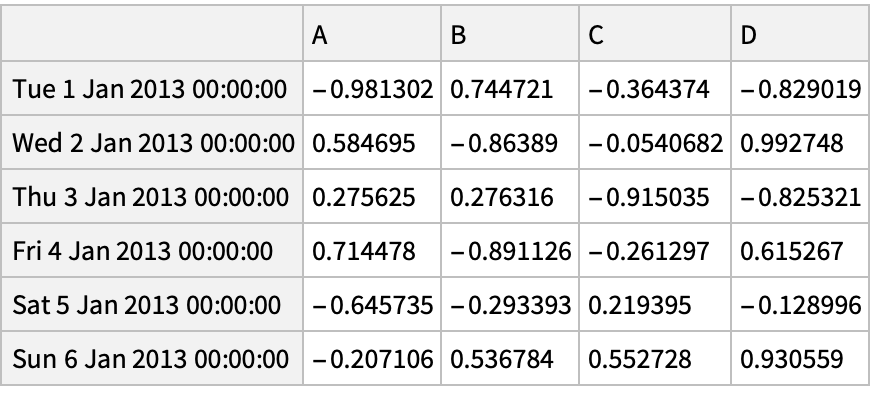
Create a "DataFrame" object:
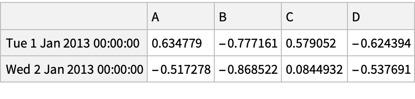
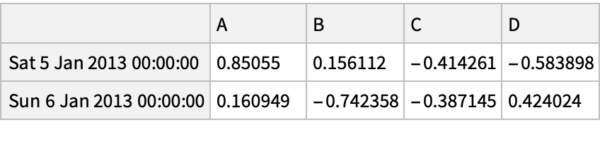
Get the preset number of top and bottom rows of the data frame:
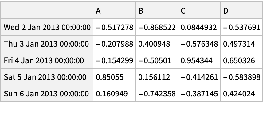
Get the specified number of top and bottom rows:
Get the index:
Alternatively:
Get column names:
Alternatively:
Get a quick statistic summary of your data:
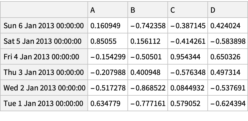
Sort by index values in descending order:
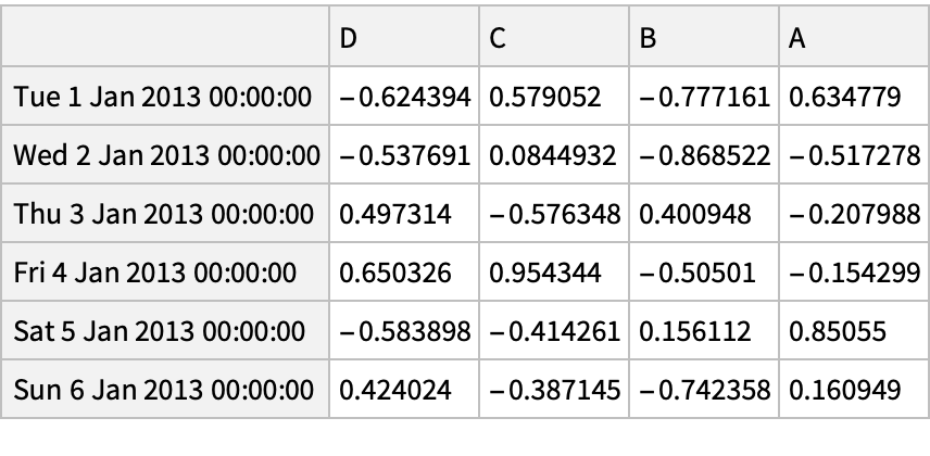
Sort by column labels in descending order:
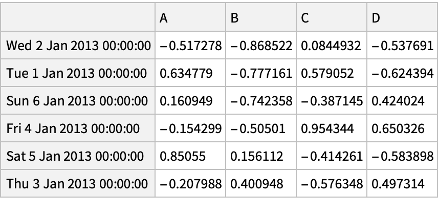
Sort by values in a column:
Transpose the data frame:
Get the dataset of the transposed values:
Convert a "DataFrame" object to a NumPy array:
Get the values in your Wolfram Language session:
Compare with the original dataset:
Selection (26)
Getting DataFrame Parts (9)
Create a new pandas object:
Select a single column, treating a column label as property. Note that the returned object is a "Series" and not a "DataFrame":
Import the "Series" object as a TimeSeries:
Plot the time series:
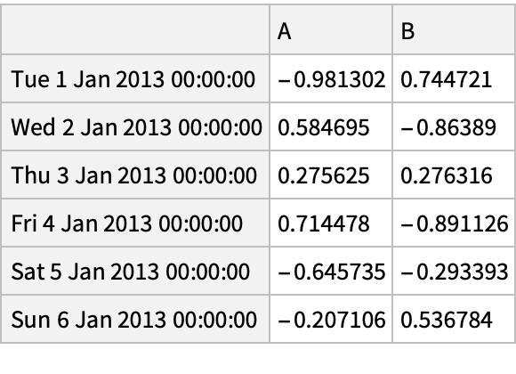
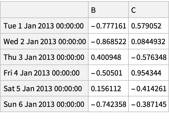
Select several columns using the "Part" syntax:
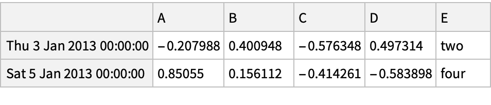
Select several rows using the Span syntax:
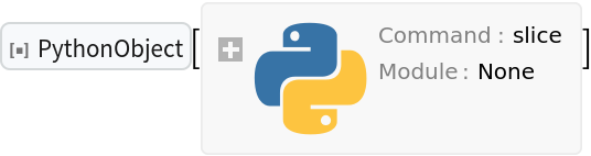
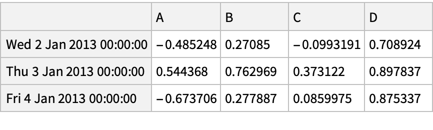
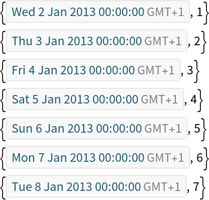
Use a Python object "Slice" to span rows by index values (rather than integer indices):
Alternatively, use the Python syntax to create a "Slice" object:
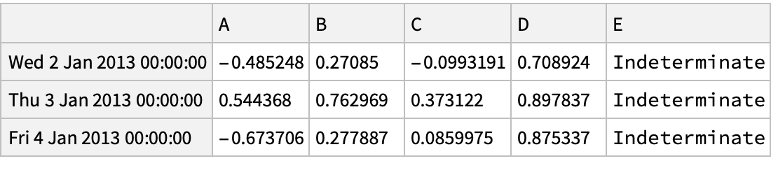
Delete rows and add a column by re-indexing:
Selecting by label (8)
Create a data frame object:
Use the "ByLabel" property of the "DataFrame" object to access values by label:
Get a cross section of the data frame using an index label:
Alternatively, use the index value:
Get a part corresponding to all rows of the specified columns (or, in the pandas parlance, select on a multi-axis by label):
Get parts of a single row in a form of a "Series" object, rather than a data frame:
Get a scalar value:
Equivalently, get fast access to a scalar using the "AtLabel" property of the "DataFrame" object:
Selecting by position (9)
Create a data frame object:
Use the "ByPosition" property of the "DataFrame" object to access values by position:
Use the Span syntax to access elements:
Select by lists of integer positions:
Slice rows explicitly:
Alternatively:
Slice columns explicitly:
Get a scalar value explicitly:
Equivalently:
Hierarchical Indexing (4)
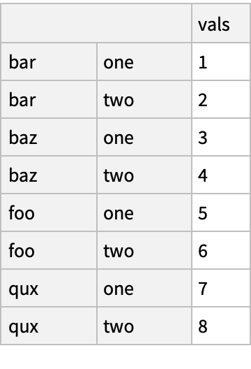
Create a "DataFrame" object for an array with more than two dimensions:
The imported "DataFrame" object is represented as an Association with keys in the form of a list:
In Python, the index is represented as a "MultiIndex" object:
Create a "MultiIndex" directly:
Boolean indexing (2)
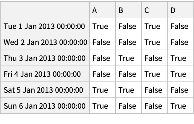
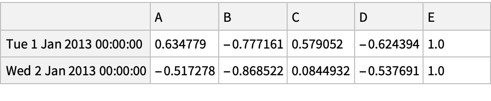
Create an array of Boolean values for which values in the column "A" are positive:
Pick rows for which the condition holds:
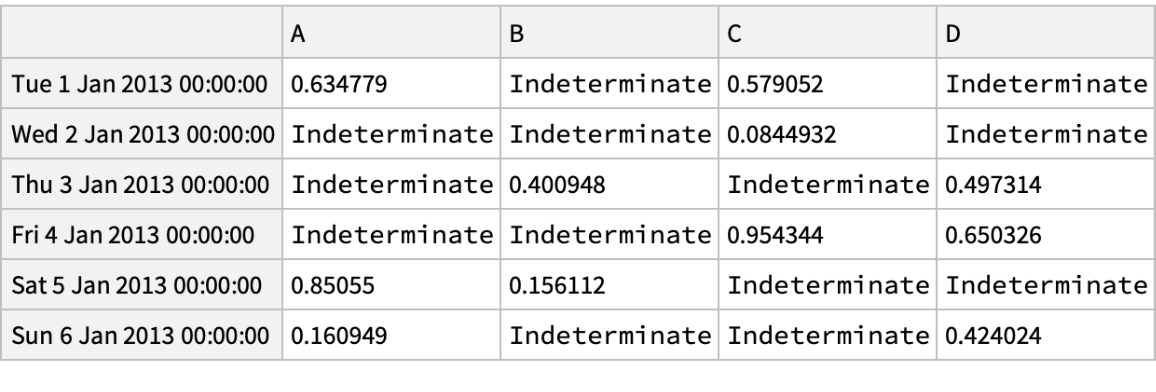
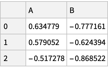
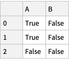
A Boolean array for positive "DataFrame" values:
Select values from a "DataFrame" where a Boolean condition is met:
Create a data frame:
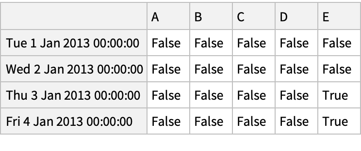
Use the "IsIn" method for filtering:
Setting Values (2)
Create a "DataFrame":
Create a new "Series" object that is longer than the "DataFrame" and starts with a time offset:
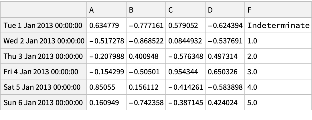
Add the object as a new column to the data frame, automatically aligning the data by the indexes:
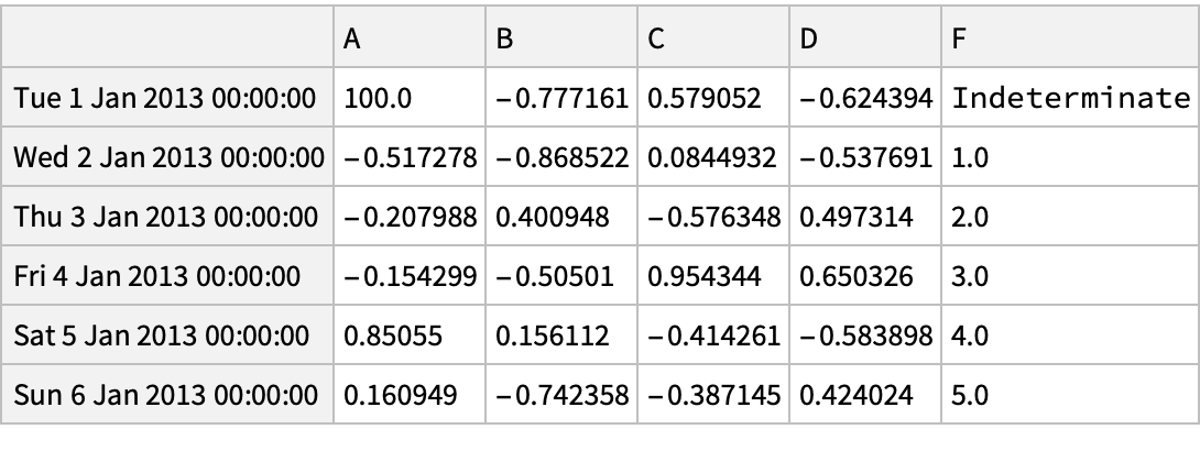
Set values by label:
Set values by position:
Set values with an array:
Create a NumPy array:
Assign a column to a NumPy array by position:
Create a "DataFrame":
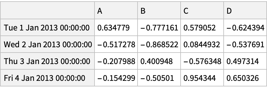
A Boolean array of values where a condition is met:
Replace values where the condition is not met:
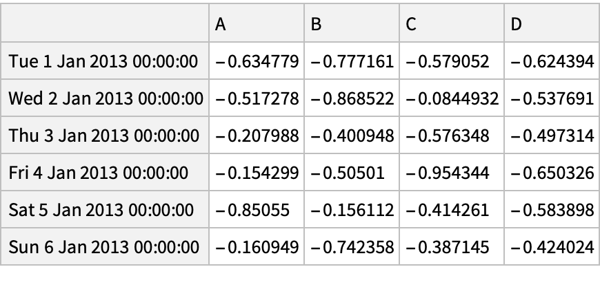
Negate positive values using the where operation with setting:
Missing data (5)
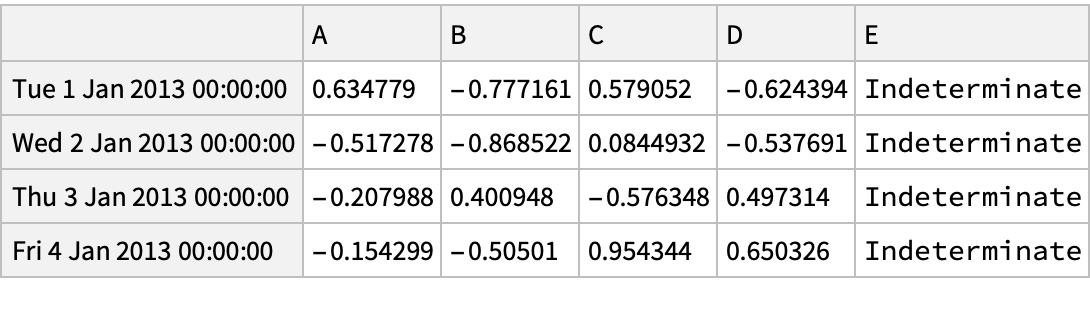
Create a "DataFrame" with missing values:
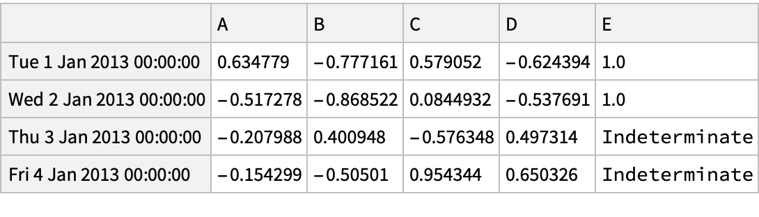
Assign some values in the "DataFrame":
Drop rows with missing data:
Fill missing data:
Get the Boolean mask where values are missing:
Binary Operations (16)
Functions vs. Operators (10)
Define a "DataFrame" object:
Add a scalar using an arithmetic operator version:
Equivalently, use a function version:
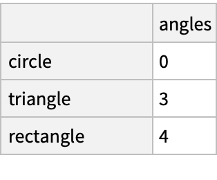
Subtract a list:
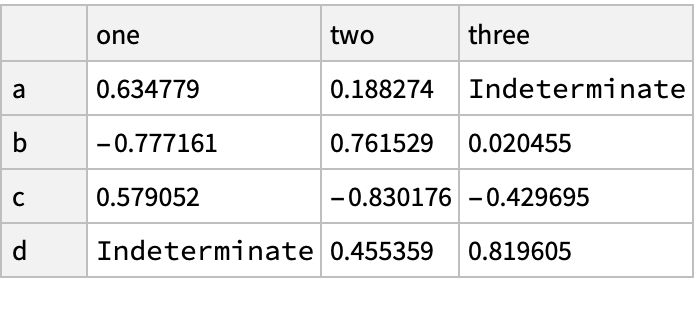
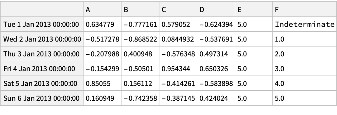
Subtract a "Series" object:
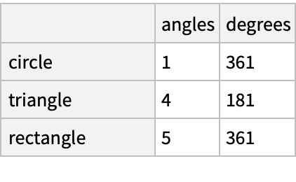
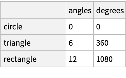
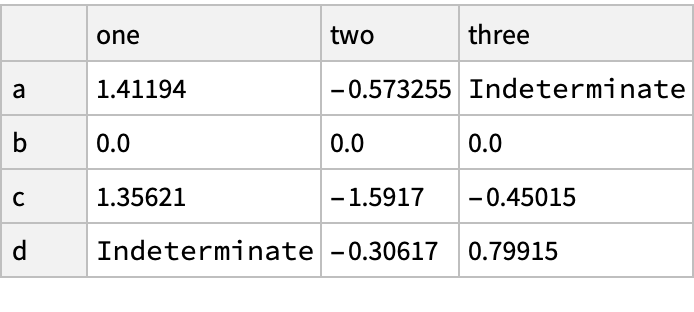
Multiply a dictionary by axis:
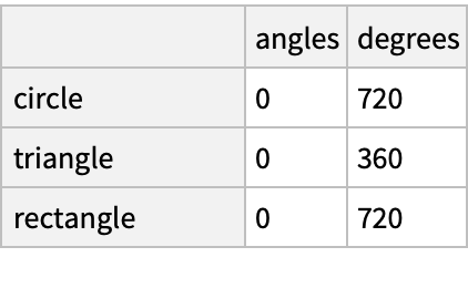
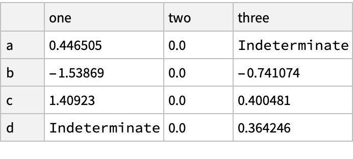
Multiply a "DataFrame" of different shape using the operator version:
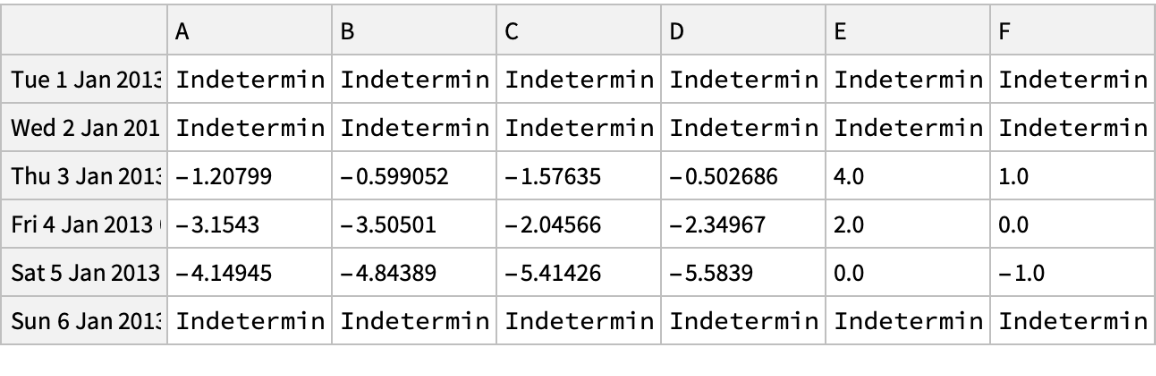
Use the function version to fill in missing values:
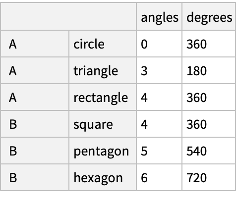
Create a "DataFrame" with a hierarchical "MultiIndex":
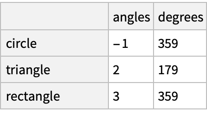
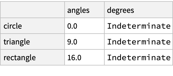
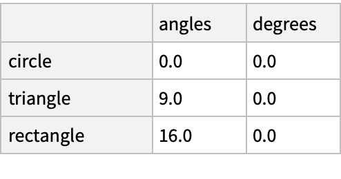
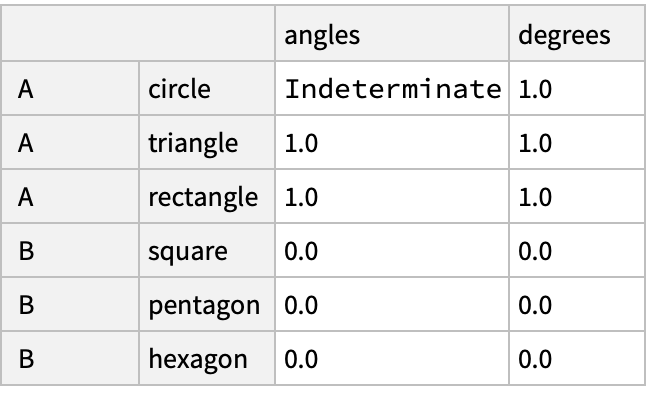
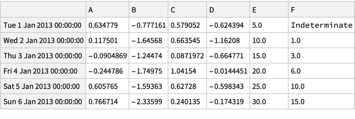
Divide by the hierarchical "DataFrame" specifying the level:
Matching / Broadcasting Behavior (6)
Create a data frame:
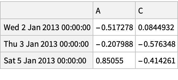
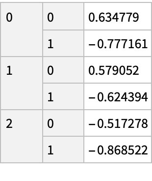
Select a row and a column:
Use the "Axis" option to match on the index or columns:
Alternatively:
Use the built-in Python divmod function with a Series object to take the floor division and modulo operation at the same time:
Do elementwise divmod:
Stats (4)
Create a data frame:
Perform descriptive statistics:
Same operation on the other axis:
Operate on objects that have different dimensionality with alignment:
Applying Functions (4)
Create a data frame:
Import a NumPy function:
Apply the function:
Create and apply a lambda function:
Histogramming (2)
Create a "Series" object:
Count unique values in the series:
String Methods (2)
Create a "Series" object:
Use the "String" attribute to operate on each element of the series:
Merging (7)
Concatenating (4)
Create a data frame:
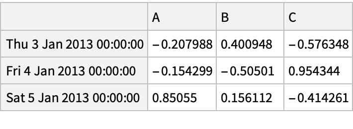
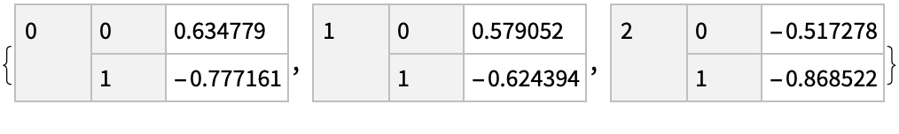
Break it into pieces:
Concatenate the pieces:
The concatenated object is the same as the original:
Database-Style Joining (3)
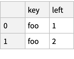
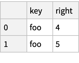
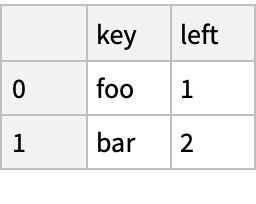
Create two "DataFrame" objects:
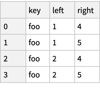
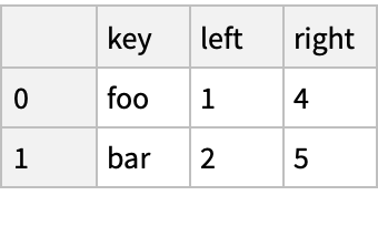
Merge the objects in SQL style:
Alternatively, with different keys:
Grouping (3)
Create a "DataFrame" object:
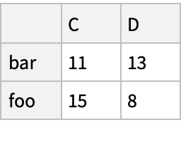
Group by values of the column "A", sum values in the groups and combine the results in a new "DataFrame" object:
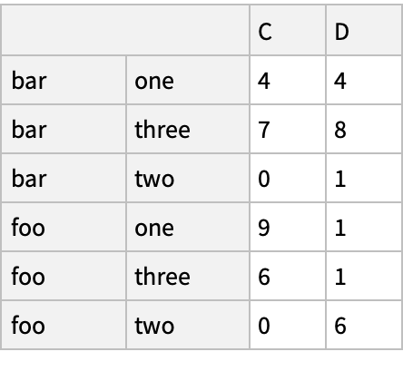
Group by multiple columns forming a hierarchical index and apply the summing function to each group:
Reshaping (5)
Pivoting (2)
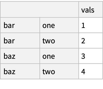
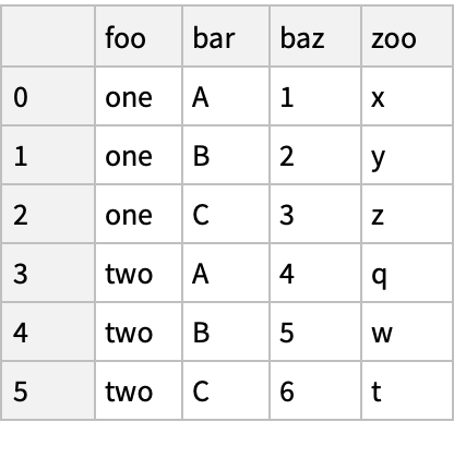
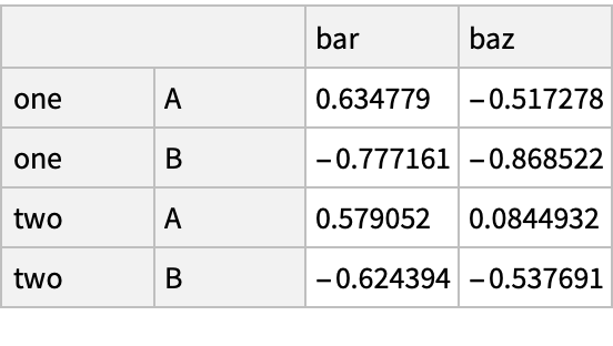
Create a "DataFrame" object:
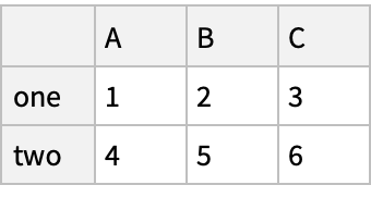
Organize the object by index and column values:
Stacking (3)
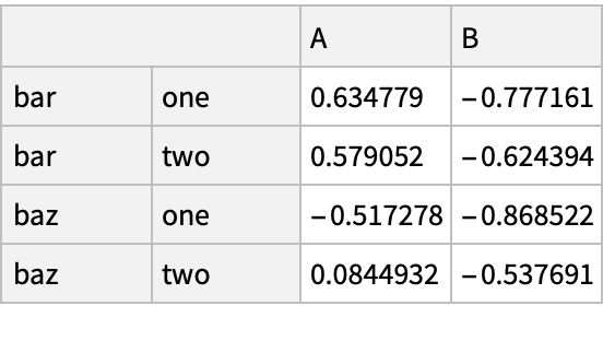
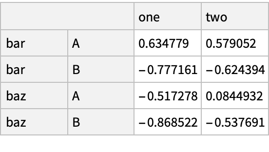
Create a "DataFrame" object with a hierarchical index:
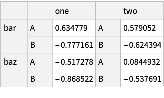
Stack the object by "compressing" a level in the columns:
Reverse the operation by "unstacking" the last level:
Time Series Resampling (3)
Create a series with 9 one-second timestamps:
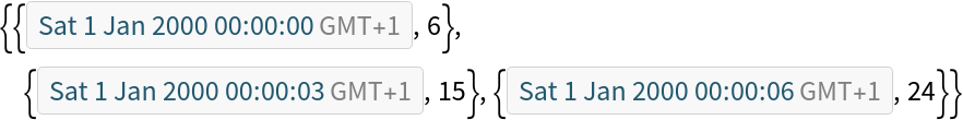
Downsample the series into 3-second bins and sum the values falling into each bin:
Check the sums:
Create a time series object with dates given in the local time zone:
Check the dates:
Localize the series to the UTC time zone and check the dates:
Convert the series to another time zone:
Create a series with quarterly frequency for a year, ending in November:
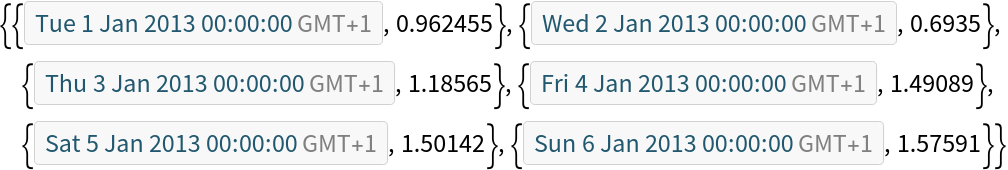
Check the start dates of a few periods in the series:
Convert the series to 9 AM of the end of the month following the quarter end and check starting dates again:
Categoricals (8)
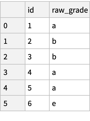
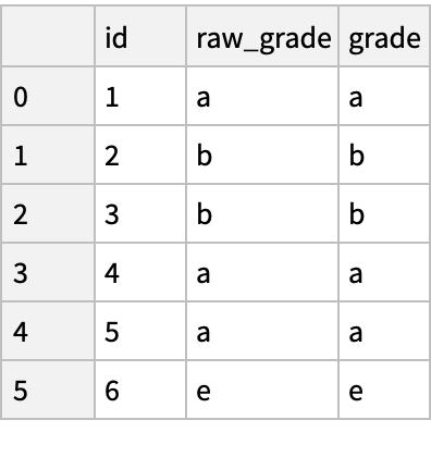
Create a "DataFrame" with a column whose values are taken from a limited alphabet:
Convert the raw grades to a categorical data type:
The current categories:
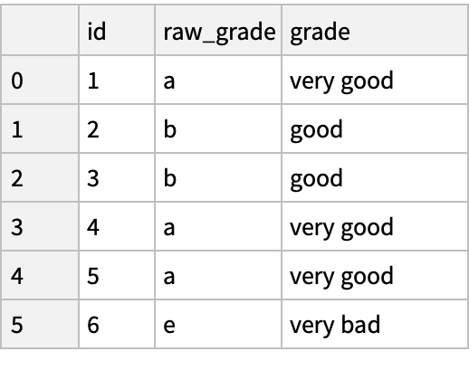
Rename the categories to more meaningful names in place:
Reorder the categories and simultaneously add the missing categories:
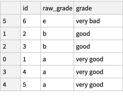
Sort by order in the categories:
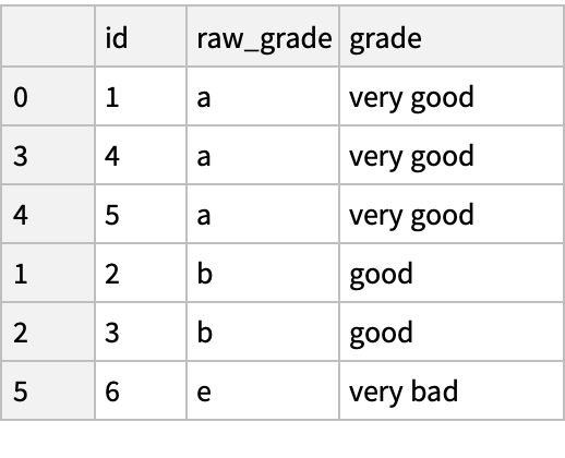
Sort by values in the "raw_grade" column (in lexicographic order):
Group by a categorical column, showing empty categories:
Plotting (5)
Construct a simple data frame object:
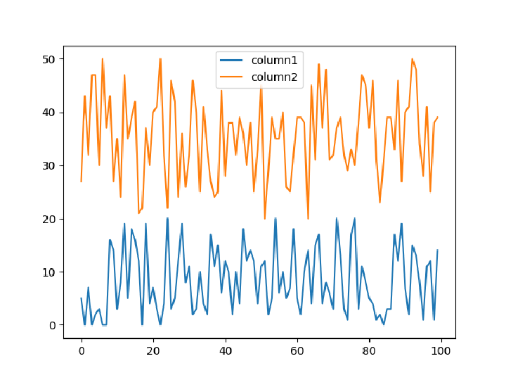
Create a plot of column values with labels:
Show the plot in the default ("PNG") format:
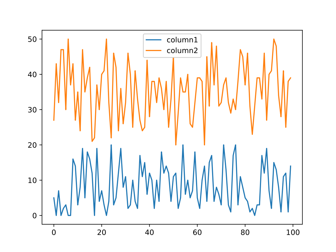
Show the plot as a vector graphics:
Export the plot to a file from Python:
Import the file:
Delete the file:
Clear the plot figure:
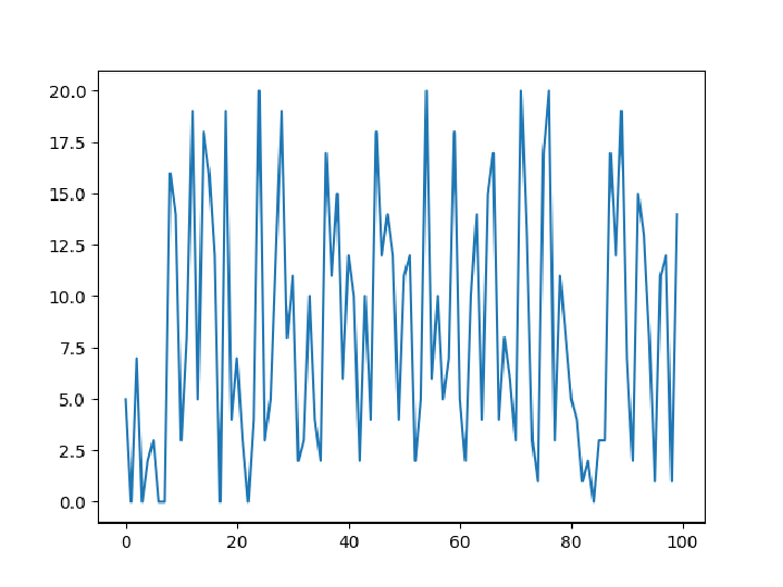
Plot the specified column:
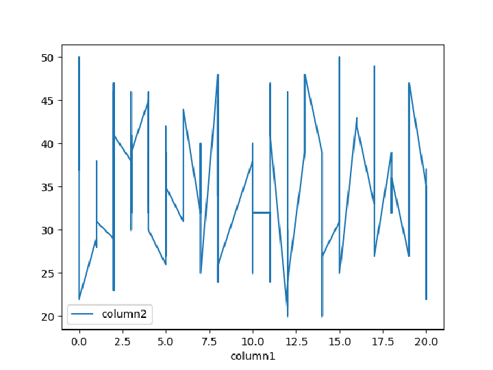
Plot one column versus another:
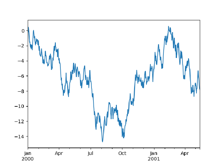
Create a time series:
Compute its cumulative sum:
Prepare a plot of the time series:
Show the plot:
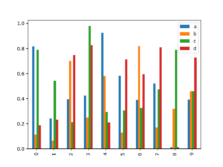
Create a data frame:
List available plot types:
Create a bar plot:
Alternatively, use the "Plot" method of the "DataFrame" object:
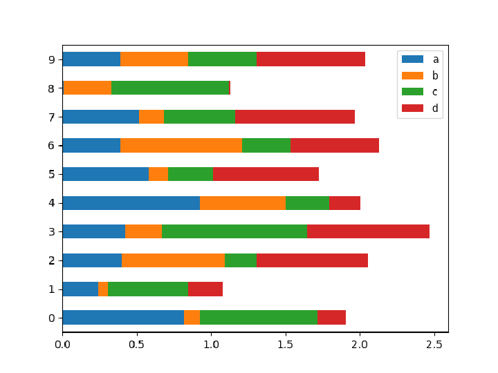
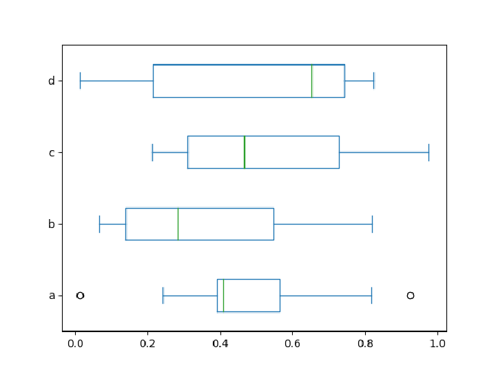
A stacked horizontal plot:
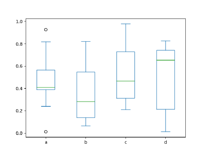
A box plot:
Pass keywords supported by the resource function MatplotlibObject "boxplot":
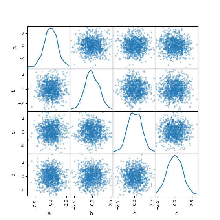
Create a data frame with normally-distributed values:
Create a scatter matrix plot using the "ScatterMatrix" method from pandas.plotting:
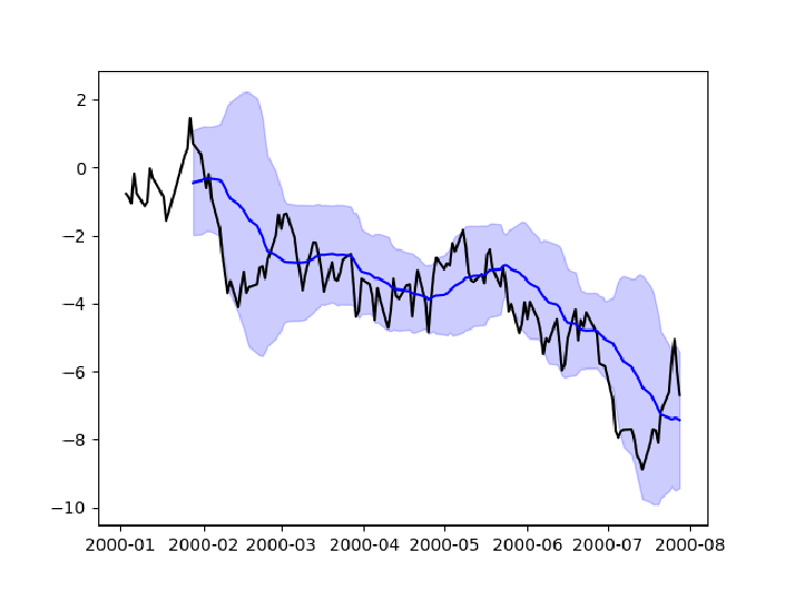
Create a time series of a cumulative random process:
Compute a moving average and standard deviation of the process:
Prepare a temporal plot of the prices, the mean values, and the Bollinger band using a MatplotlibObject:
Show the plots:
Importing and exporting data (9)
CSV (4)
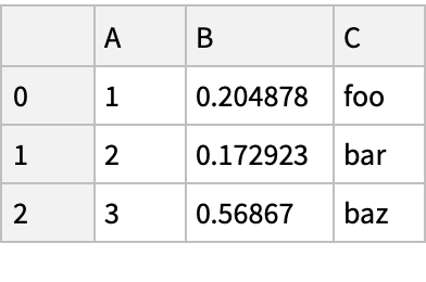
Write to a CSV file:
Print contents of the file:
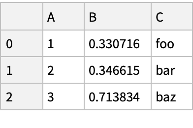
Read the CSV file as a "DataFrame" object:
Clean up:
problematic in 2.2.0:
Excel (5)
Create a new pandas object:
Write to an Excel file:
Check the file:
Read the file as "DataFrame":
Clean up:
Properties and Relations (7)
PandasObject[…] gives the same result as the resource function PythonObject with a special configuration:
Get information on a pandas object:
Open the user guide in your default web browser:
Some of the functions and classes available in the pandas module:
Information on a class:
The web documentation for a class:
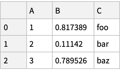
pandas’s "DataFrame" is analogous to Dataset, but keeps the object on the Python side:
Print the object in Python:
Transfer the data from Python to create a Dataset:
Many pandas operations are parallel to operations on Dataset:
Select rows satisfying a condition:
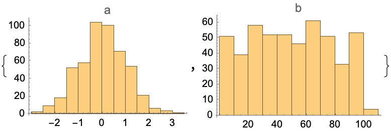
Plot histograms of the columns:
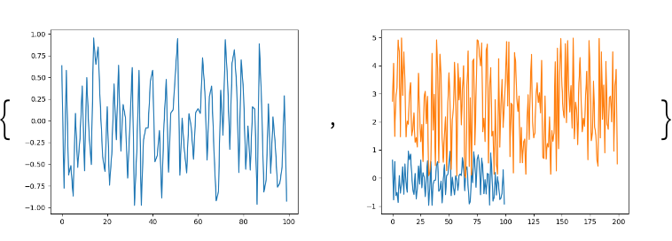
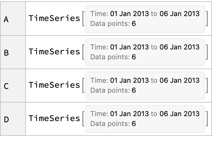
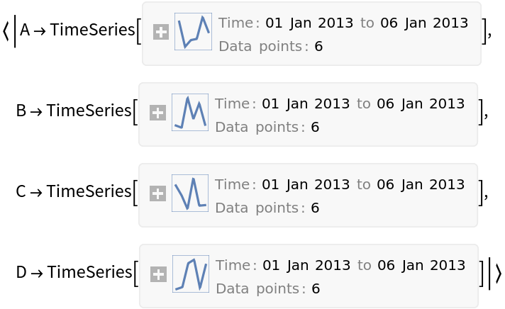
Similarly, pandas’s "Series" object is analogous to TimeSeries:
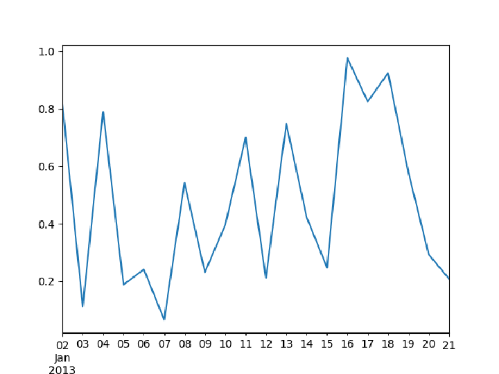
Plot the time series in Python:
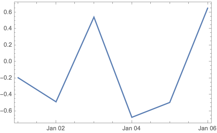
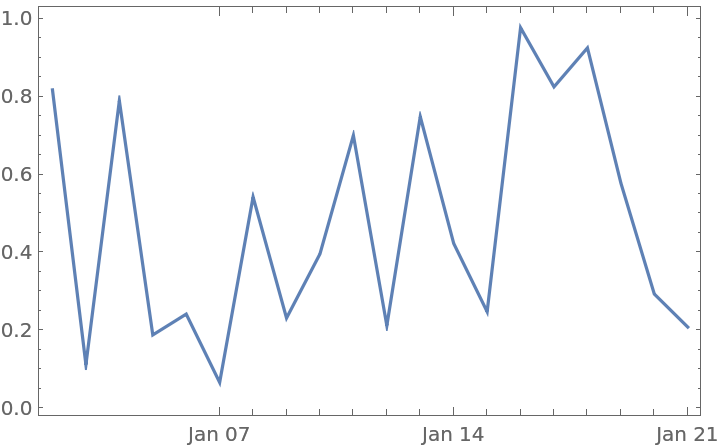
Plot the imported time series with DateListPlot:
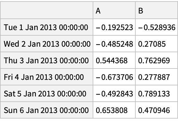
Create a "DataFrame" and a Boolean mask for positive values:
PythonObject allows you to apply Python commands directly, and bring the results back to the Wolfram Language if necessary:
Alternatively:
Possible Issues (2)
Create a pandas object:
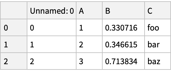
Since NumPy arrays have a single data type for the entire array (dtype), importing a NumPy array to the Wolfram Language may fail if one of the columns cannot be imported directly:
Drop the problematic column to import only numeric values:
Import the rest:
Alternatively, import the entire array by converting the NumPy array to list:
Create two "Series" objects:
The Matplotlib library, used by pandas, accumulates the results of successive plot commands:
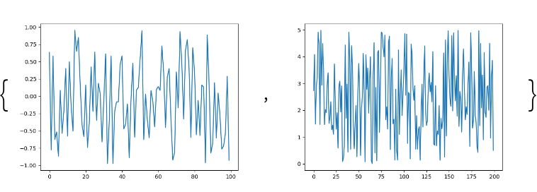
Clear the plot figure to create separate plots instead:

![(titanic = pd["ReadCSV"[
"https://raw.githubusercontent.com/datasciencedojo/datasets/master/titanic.csv"]]) // Normal](https://www.wolframcloud.com/obj/resourcesystem/images/52c/52c488d5-cc0c-4116-bbbe-aa35b6c7fc92/04c218e2c3d9a848.png)
![titanic["Aggregate"[<|"Age" -> {"min", "max", "median", "skew"}, "Fare" -> {"min", "max", "median", "mean"}|>]] // Normal](https://www.wolframcloud.com/obj/resourcesystem/images/52c/52c488d5-cc0c-4116-bbbe-aa35b6c7fc92/624aca77b4dd938d.png)


![pd["DataFrame"[RandomReal[{-1, 1}, {6, 4}], "Index" -> dates, "Columns" -> CharacterRange["A", "D"]]]](https://www.wolframcloud.com/obj/resourcesystem/images/52c/52c488d5-cc0c-4116-bbbe-aa35b6c7fc92/28e8de0c96a6ccb5.png)
![pd["DataFrame"[<|
"A" -> 1.0,
"B" -> pd["Timestamp"["20130102"]],
"C" -> pd["Series"[1, "index" -> Range[0, 3], "dtype" -> "float32"]],
"D" -> ConstantArray[0, 4],
"E" -> pd["Categorical"[{"test", "train", "test", "train"}]],
"F" -> "foo"|>]]](https://www.wolframcloud.com/obj/resourcesystem/images/52c/52c488d5-cc0c-4116-bbbe-aa35b6c7fc92/738a0e5fec5e1b0b.png)
![df = pd["DataFrame"[RandomReal[{-1, 1}, {6, 4}], "Index" -> pd["DateRange"["20130101", "Periods" -> 6]], "Columns" -> CharacterRange["A", "D"]]]](https://www.wolframcloud.com/obj/resourcesystem/images/52c/52c488d5-cc0c-4116-bbbe-aa35b6c7fc92/5ed5e045b3b6218e.png)


![df = pd["DataFrame"[RandomReal[{-1, 1}, {6, 4}], "Index" -> pd["DateRange"["20130101", "Periods" -> 6]], "Columns" -> CharacterRange["A", "D"]]]](https://www.wolframcloud.com/obj/resourcesystem/images/52c/52c488d5-cc0c-4116-bbbe-aa35b6c7fc92/72e4fd9f916d5703.png)


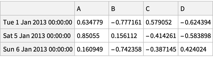
![(df = pd[
"DataFrame"[RandomReal[{-1, 1}, {6, 4}], "Index" -> dates, "Columns" -> CharacterRange["A", "D"]]]) // Normal](https://www.wolframcloud.com/obj/resourcesystem/images/52c/52c488d5-cc0c-4116-bbbe-aa35b6c7fc92/20cb74dab630070d.png)
![(df = pd[
"DataFrame"[RandomReal[{-1, 1}, {6, 4}], "Index" -> pd["DateRange"["20130101", "Periods" -> 6]], "Columns" -> CharacterRange["A", "D"]]]) // Normal](https://www.wolframcloud.com/obj/resourcesystem/images/52c/52c488d5-cc0c-4116-bbbe-aa35b6c7fc92/12602408ef70078a.png)


![df = pd["DataFrame"[<|"vals" -> Range[4]|>, "Index" -> {{"bar", "bar", "baz", "baz"}, {"one", "two", "one", "two"}}]]](https://www.wolframcloud.com/obj/resourcesystem/images/52c/52c488d5-cc0c-4116-bbbe-aa35b6c7fc92/6d00d88f954ca1a8.png)
![(df = pd[
"DataFrame"[RandomReal[{-1, 1}, {6, 4}], "Index" -> pd["DateRange"["20130101", "Periods" -> 6]], "Columns" -> CharacterRange["A", "D"]]]) // Normal](https://www.wolframcloud.com/obj/resourcesystem/images/52c/52c488d5-cc0c-4116-bbbe-aa35b6c7fc92/52f210255e3471f7.png)

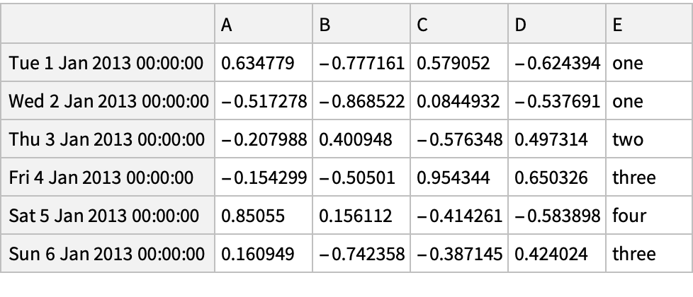
![(df = pd[
"DataFrame"[
Join[RandomReal[{-1, 1}, {6, 4}], List /@ {"one", "one", "two", "three", "four", "three"}, 2], "Index" -> pd["DateRange"["20130101", "Periods" -> 6]], "Columns" -> CharacterRange["A", "E"]]]) // Normal](https://www.wolframcloud.com/obj/resourcesystem/images/52c/52c488d5-cc0c-4116-bbbe-aa35b6c7fc92/0fe7f8ada7c34453.png)
![(df = pd[
"DataFrame"[RandomReal[{-1, 1}, {6, 4}], "Index" -> pd["DateRange"["20130101", "Periods" -> 6]], "Columns" -> CharacterRange["A", "D"]]]) // Normal](https://www.wolframcloud.com/obj/resourcesystem/images/52c/52c488d5-cc0c-4116-bbbe-aa35b6c7fc92/07123faa775a5846.png)


![(df = pd[
"DataFrame"[RandomReal[{-1, 1}, {6, 4}], "Index" -> pd["DateRange"["20130101", "Periods" -> 6]], "Columns" -> CharacterRange["A", "D"]]]) // Normal](https://www.wolframcloud.com/obj/resourcesystem/images/52c/52c488d5-cc0c-4116-bbbe-aa35b6c7fc92/75c4ff62fd5805eb.png)


![(df = pd[
"DataFrame"[RandomReal[{-1, 1}, {4, 4}], "Index" -> pd["DateRange"["20130101", "Periods" -> 4]], "Columns" -> CharacterRange["A", "D"]]]) // Normal](https://www.wolframcloud.com/obj/resourcesystem/images/52c/52c488d5-cc0c-4116-bbbe-aa35b6c7fc92/24133f7d2ee1f993.png)


![(dfm = pd[
"DataFrame"[<|"angles" -> {0, 3, 4, 4, 5, 6}, "degrees" -> {360, 180, 360, 360, 540, 720}|>, "Index" -> {{" A", " A", " A", " B", " B", " B"}, {"circle", "triangle", "rectangle", "square", "pentagon", "hexagon"}}]]) // Normal](https://www.wolframcloud.com/obj/resourcesystem/images/52c/52c488d5-cc0c-4116-bbbe-aa35b6c7fc92/04fabafdb2649aa0.png)
![(df = pd["DataFrame"[<|
"one" -> pd["Series"[RandomReal[{-1, 1}, {3}], "Index" -> {"a", "b", "c"}]], "two" -> pd["Series"[RandomReal[{-1, 1}, {4}], "Index" -> {"a", "b", "c", "d"}]],
"three" -> pd["Series"[RandomReal[{-1, 1}, {3}], "Index" -> {"b", "c", "d"}]]
|>
]]) // Normal](https://www.wolframcloud.com/obj/resourcesystem/images/52c/52c488d5-cc0c-4116-bbbe-aa35b6c7fc92/77d3ceb8a482bc00.png)


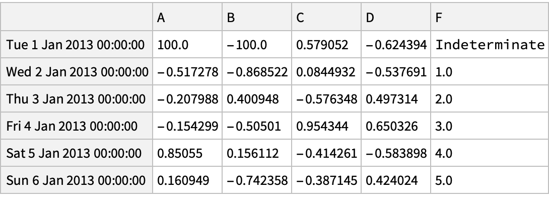
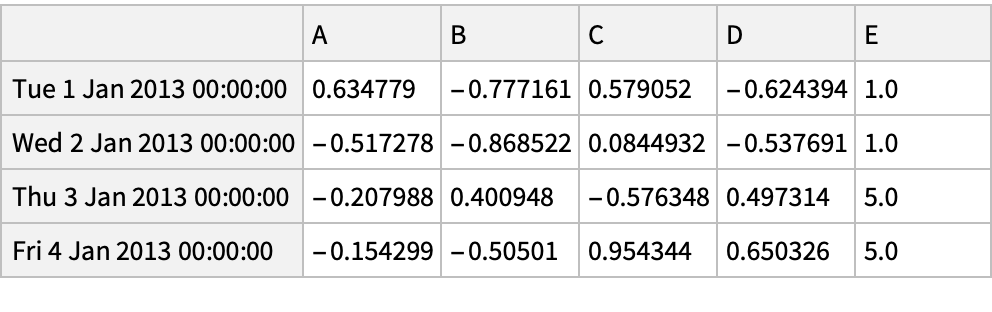
![(df = pd[
"DataFrame"[
Join[RandomReal[{-1, 1}, {6, 4}], Table[{5}, {6}], List /@ Flatten[{None, Range[5]}], 2], "Index" -> pd["DateRange"["20130101", "Periods" -> 6]], "Columns" -> CharacterRange["A", "F"]]]) // Normal](https://www.wolframcloud.com/obj/resourcesystem/images/52c/52c488d5-cc0c-4116-bbbe-aa35b6c7fc92/012b8b61f38fcbb0.png)


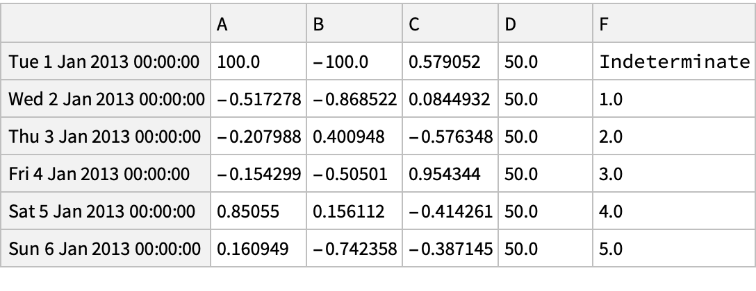
![(df = pd[
"DataFrame"[
Join[RandomReal[{-1, 1}, {6, 4}], Table[{5}, {6}], List /@ Flatten[{None, Range[5]}], 2], "Index" -> pd["DateRange"["20130101", "Periods" -> 6]], "Columns" -> CharacterRange["A", "F"]]]) // Normal](https://www.wolframcloud.com/obj/resourcesystem/images/52c/52c488d5-cc0c-4116-bbbe-aa35b6c7fc92/479bf79692a487b3.png)


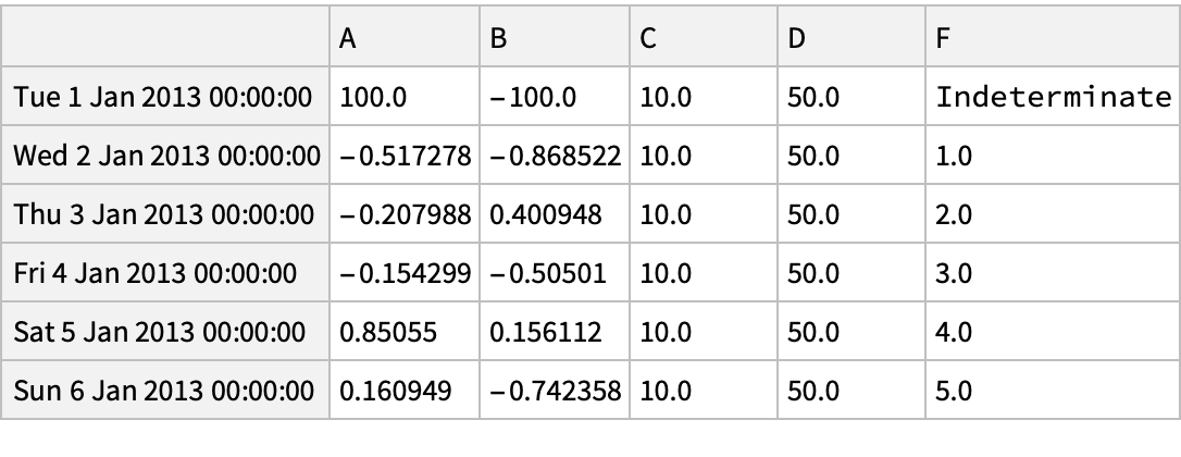
![(df = pd[
"DataFrame"[<|
"A" -> {"foo", "bar", "foo", "bar", "foo", "bar", "foo", "foo"},
"B" -> {"one", "one", "two", "three", "two", "two", "one", "three"},
"C" -> RandomInteger[10, {8}],
"D" -> RandomInteger[10, {8}]
|>]]) // Normal](https://www.wolframcloud.com/obj/resourcesystem/images/52c/52c488d5-cc0c-4116-bbbe-aa35b6c7fc92/2daf32d6aa207a02.png)

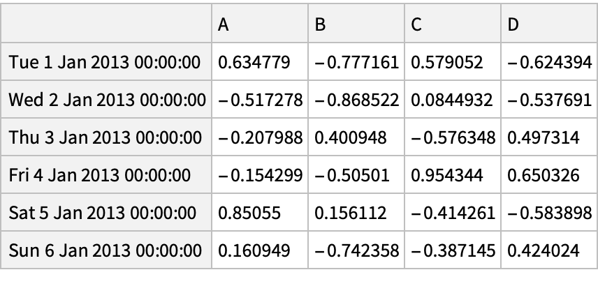
![(df = pd[
"DataFrame"[<|"foo" -> {"one", "one", "one", "two", "two", "two"},
"bar" -> {"A", "B", "C", "A", "B", "C"}, "baz" -> Range[6], "zoo" -> {"x", "y", "z", "q", "w", "t"}|>]]) // Normal](https://www.wolframcloud.com/obj/resourcesystem/images/52c/52c488d5-cc0c-4116-bbbe-aa35b6c7fc92/30cd96428dba5c60.png)
![(df = pd[
"DataFrame"[RandomReal[{-1, 1}, {4, 2}], "Index" -> {{"bar", "bar", "baz", "baz"}, {"one", "two", "one", "two"}}, "Columns" -> {"A", "B"}]]) // Normal](https://www.wolframcloud.com/obj/resourcesystem/images/52c/52c488d5-cc0c-4116-bbbe-aa35b6c7fc92/6a610c5641df5dc2.png)


![s["Assign"[
"index" -> (periods[
"AsFrequency"["Frequency" -> "M", "how" -> "e"]] + 1)[
"AsFrequency"["Frequency" -> "H", "how" -> "s"]] + 9]]](https://www.wolframcloud.com/obj/resourcesystem/images/52c/52c488d5-cc0c-4116-bbbe-aa35b6c7fc92/3ac1e317babb184b.png)

![(df = pd[
"DataFrame"[<|"id" -> {1, 2, 3, 4, 5, 6}, "raw_grade" -> {"a", "b", "b", "a", "a", "e"}|>]]) // Normal](https://www.wolframcloud.com/obj/resourcesystem/images/52c/52c488d5-cc0c-4116-bbbe-aa35b6c7fc92/5173ba3b5cc8a805.png)

![df = pd["DataFrame"[<|"column1" -> RandomInteger[{0, 20}, n], "column2" -> RandomInteger[{20, 50}, n]|>]]](https://www.wolframcloud.com/obj/resourcesystem/images/52c/52c488d5-cc0c-4116-bbbe-aa35b6c7fc92/162a3f25eab9822b.png)


![df = pd["DataFrame"[
RandomVariate[NormalDistribution[0, 1], {1000, 4}], "columns" -> CharacterRange["a", "d"]]]](https://www.wolframcloud.com/obj/resourcesystem/images/52c/52c488d5-cc0c-4116-bbbe-aa35b6c7fc92/2540ded5bee6065e.png)

![price = pd[
"Series"[FoldList[Plus, RandomReal[{-1, 1}, {150}]], "Index" -> pd["DateRange"["2000-1-1", "Periods" -> 150, "Frequency" -> "B"]]]]](https://www.wolframcloud.com/obj/resourcesystem/images/52c/52c488d5-cc0c-4116-bbbe-aa35b6c7fc92/412646fe239b7ee3.png)


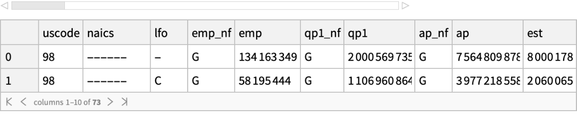
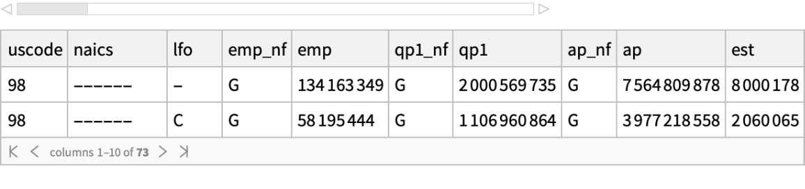
![fname = ExtractArchive[
"https://www2.census.gov/programs-surveys/cbp/datasets/2020/cbp20us.zip", $TemporaryDirectory] // First;](https://www.wolframcloud.com/obj/resourcesystem/images/52c/52c488d5-cc0c-4116-bbbe-aa35b6c7fc92/7048792963c4b2f8.png)


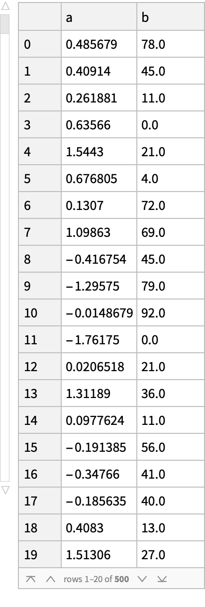
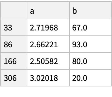
![df = pd["DataFrame"[<|
"a" -> RandomVariate[NormalDistribution[0, 1], {n}], "b" -> RandomInteger[100, {n}]|>]]](https://www.wolframcloud.com/obj/resourcesystem/images/52c/52c488d5-cc0c-4116-bbbe-aa35b6c7fc92/61e9696d0b8bc345.png)


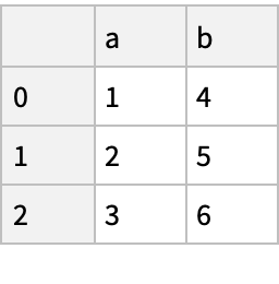
![(df = pd["DataFrame"[<|
"A" -> Range[3],
"B" -> RandomReal[1, {3}],
"C" -> {"foo", "bar", "baz"}
|>
]]) // Normal](https://www.wolframcloud.com/obj/resourcesystem/images/52c/52c488d5-cc0c-4116-bbbe-aa35b6c7fc92/7e0fefb223a74e50.png)