Wolfram Function Repository
Instant-use add-on functions for the Wolfram Language
Function Repository Resource:
Compute the evolute of a curve
ResourceFunction["EvoluteCurve"][c,t] computes the evolute of the curve c. |
Define the curve of an ellipse:
| In[1]:= |
Compute its evolute:
| In[2]:= |
| Out[2]= |
Plot the ellipse and evolute:
| In[3]:= | ![\[Alpha] = ellipse[3/2, 1, t];
\[Epsilon] = ResourceFunction["EvoluteCurve"][\[Alpha], t];
ParametricPlot[Evaluate[{\[Alpha], \[Epsilon]}], {t, 0, 2 \[Pi]}]](https://www.wolframcloud.com/obj/resourcesystem/images/44a/44a7a838-51b2-4a43-8559-5ed3361e2c58/0433039577ddff90.png) |
| Out[3]= | 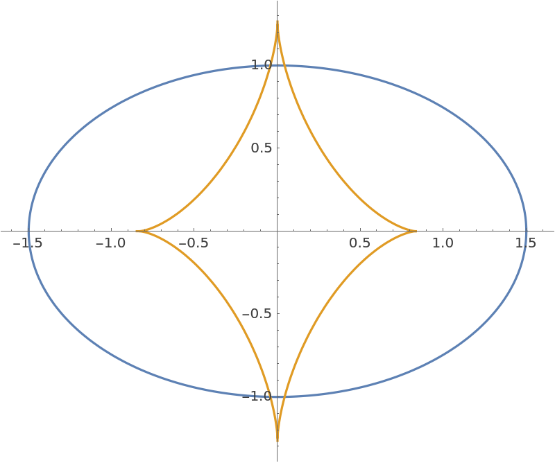 |
Define a curve known as a tractrix:
| In[4]:= |
Its evolute is a catenary:
| In[5]:= |
| Out[5]= |
Plot the result:
| In[6]:= | ![\[Alpha] = tractrix[1, t];
\[Epsilon] = ResourceFunction["EvoluteCurve"][\[Alpha], t];
ParametricPlot[{\[Alpha], \[Epsilon]}, {t, 0.01, \[Pi]}, Axes -> None]](https://www.wolframcloud.com/obj/resourcesystem/images/44a/44a7a838-51b2-4a43-8559-5ed3361e2c58/7a3c049ba1b2057d.png) |
| Out[6]= | 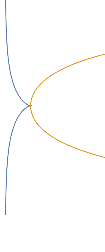 |
Define a curve called a cissoid:
| In[7]:= |
Plot repeated evolutes of the curve:
| In[8]:= |
| Out[8]= | 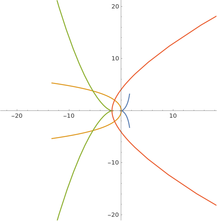 |
Evolute of a cycloid:
| In[9]:= |
| In[10]:= |
| Out[10]= |
A cycloidal pendulum, which exhibits the tautochrone property:
| In[11]:= | ![Module[{y, z}, \[Delta] = cycloid[-1]; y[a_] = {Thickness[.008], Line[{\[Delta][a], ResourceFunction["EvoluteCurve"][\[Delta][a], a]}],
PointSize[.05], Point[\[Delta][a]]}; z[a_] := ParametricPlot[
Evaluate[{\[Delta][t], ResourceFunction["EvoluteCurve"][\[Delta][t], t]}], {t, -.001, 2 \[Pi] + .001}, Epilog -> y[a], Axes -> None];
GraphicsGrid[Table[z[(3 a + b) \[Pi]/7], {a, 0, 3}, {b, 3}]]]](https://www.wolframcloud.com/obj/resourcesystem/images/44a/44a7a838-51b2-4a43-8559-5ed3361e2c58/0055e6b65608a78a.png) |
| Out[11]= | 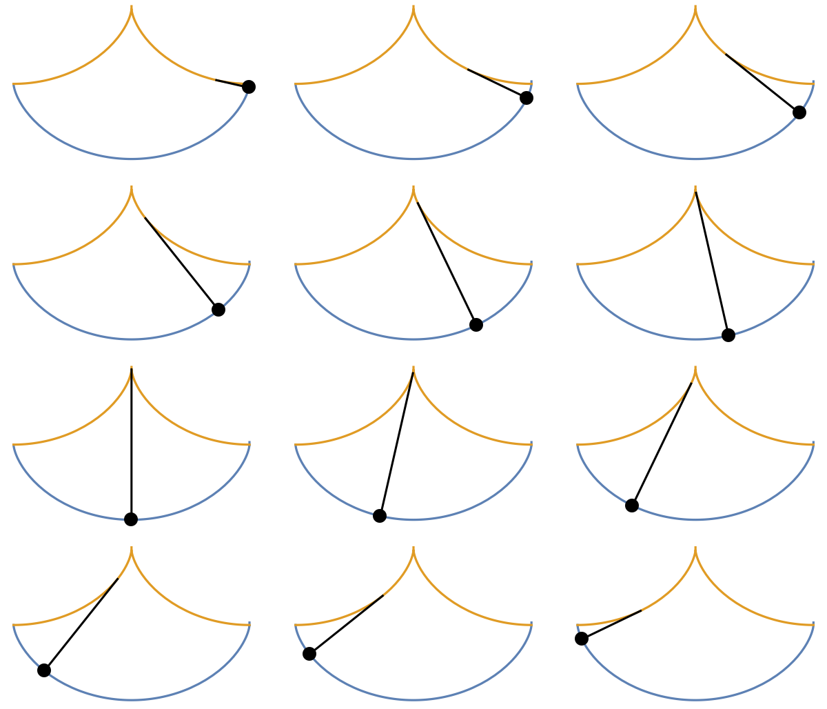 |
The evolute of a curve can be expressed in terms of the curvature and the normal vector:
| In[12]:= | ![ResourceFunction["EvoluteCurve"][{f[t], g[t]}, t] == {f[t], g[t]} + ResourceFunction["NormalVector"][{f[t], g[t]}, t]/
ResourceFunction["Curvature"][{f[t], g[t]}, t] // Simplify](https://www.wolframcloud.com/obj/resourcesystem/images/44a/44a7a838-51b2-4a43-8559-5ed3361e2c58/2929934060f94003.png) |
| Out[12]= |
Show the evolute as an envelope of normals:
| In[13]:= | ![cardioid[a_][t_] = Entity["PlaneCurve", "Cardioid"][
EntityProperty["PlaneCurve", "ParametricEquations"]][a][t];
cev[a_][t_] = ResourceFunction["EvoluteCurve"][cardioid[a][t], t] // Simplify;
nv[a_][t_] = ResourceFunction["NormalVector"][cardioid[a][t], t] // Simplify;](https://www.wolframcloud.com/obj/resourcesystem/images/44a/44a7a838-51b2-4a43-8559-5ed3361e2c58/445febfa55e4c6be.png) |
| In[14]:= | ![With[{a = 1}, ParametricPlot[{cardioid[a][t], cev[a][t]}, {t, 0, 2 \[Pi]}, PlotStyle -> {Thick, Directive[Thick, Dashed]}, Epilog -> {Directive[Opacity[0.3], Dashed], Table[InfiniteLine[cardioid[a][t], nv[a][t]], {t, \[Pi]/25, 2 \[Pi] - \[Pi]/25, \[Pi]/25}]}]]](https://www.wolframcloud.com/obj/resourcesystem/images/44a/44a7a838-51b2-4a43-8559-5ed3361e2c58/040c7b4735ee5511.png) |
| Out[14]= | 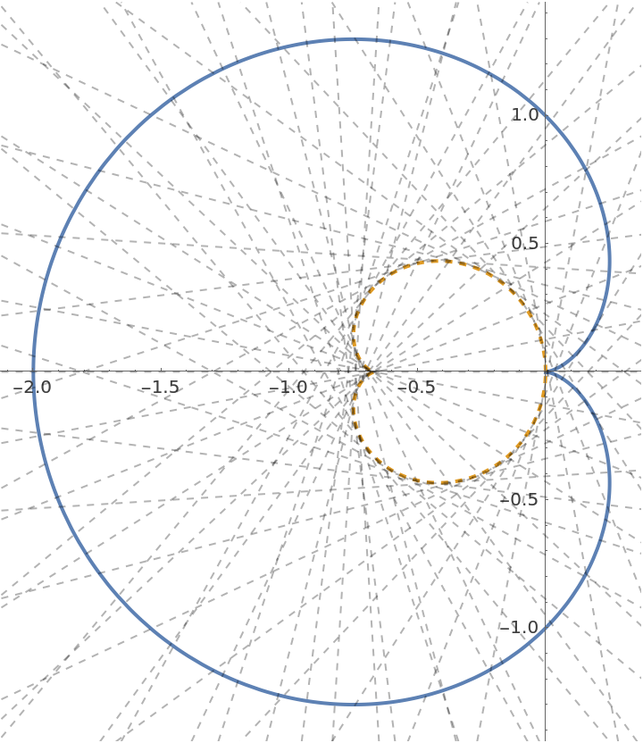 |
This work is licensed under a Creative Commons Attribution 4.0 International License