Basic Examples (3)
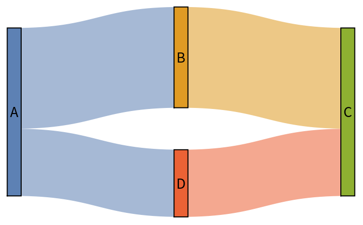
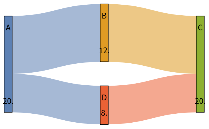
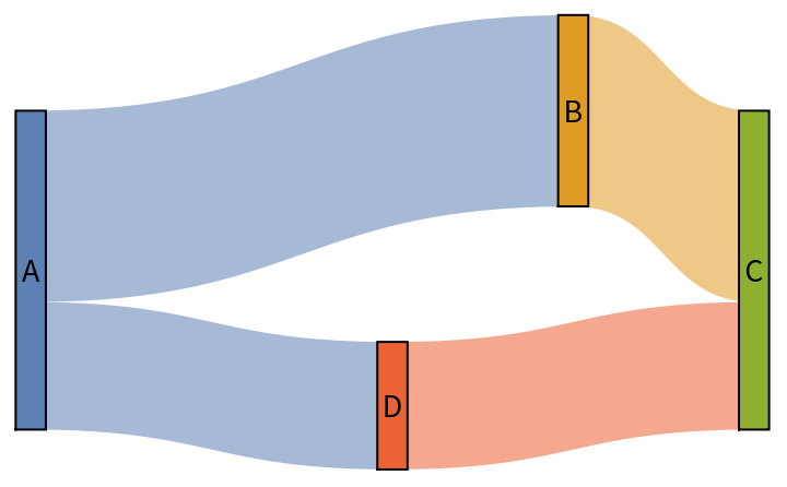
A simple diamond-shaped flow network: one source splits two ways, then re-merges:
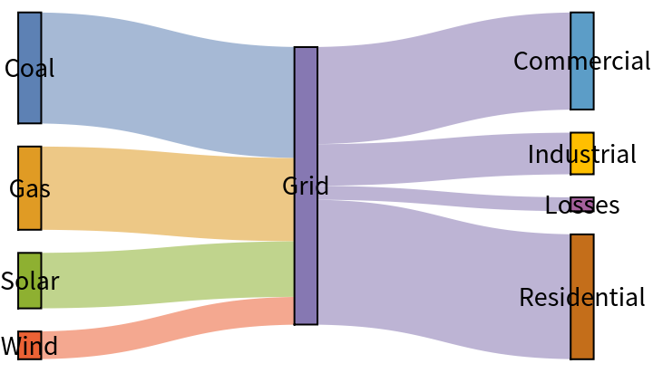
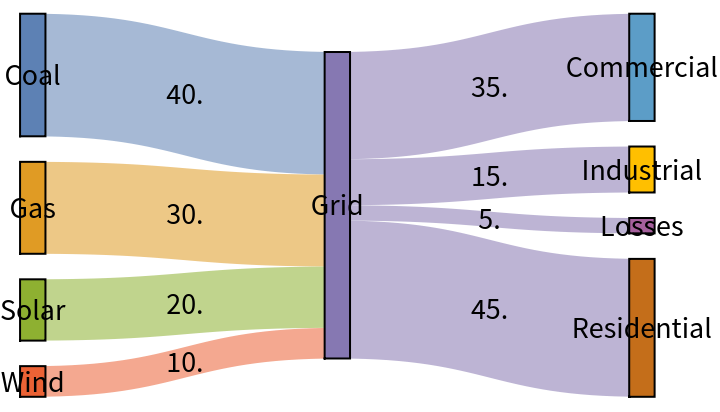
A many-to-one-to-many network: four power sources feed a single grid hub, which fans out to four consumer categories:
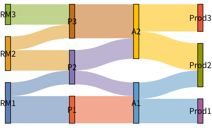
A four-layer manufacturing network (raw materials -> processing -> assembly -> products), with cross-wiring between layers:
Scope (3)
SankeyChart will interpret a square matrix of integers as a WeightedAdjacenecyGraph, with zero or Infinity indicating no flow. The vertices will be labeled 1,2,…,n unless you provide a "VertexLabels":
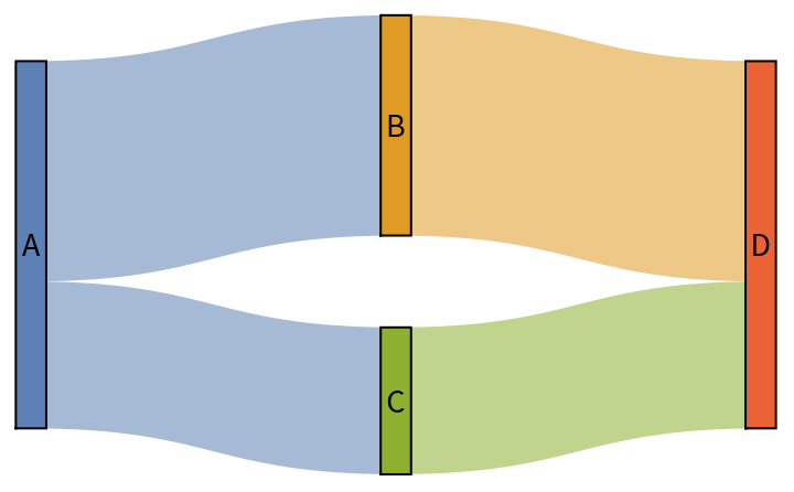
SankeyChart can also accept OptimimFlowData objects generated by FundMaximalFlow:
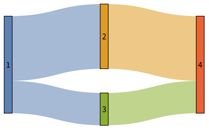
"Backflow" is supported:
Options (20)
EdgeOrigin (1)
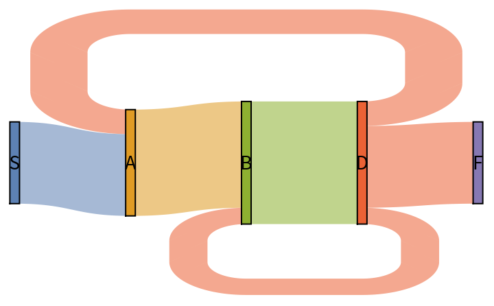
Controls which side sources are drawn on -- Left, Right, Top, or Bottom -- and hence which direction flow travels across the page:
"VertexLabelPosition" (2)
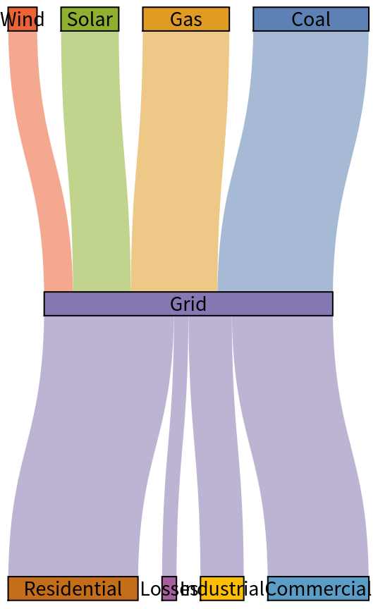
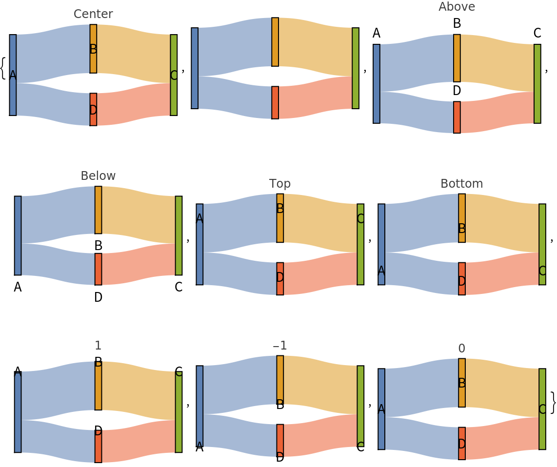
By default only the vertex name is shown (centered) but "VertexLabelPosition" can take values None, Above, Below, Top, Bottom or a number:
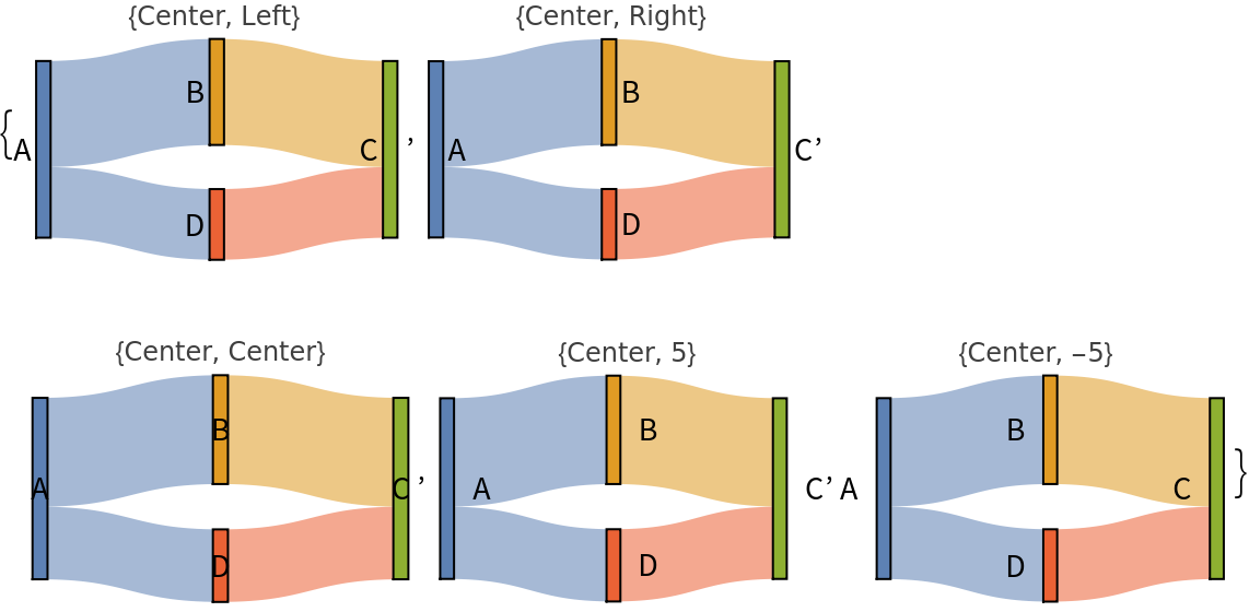
"VertexLabelPositon" can also take a second value for the alternate dimension:
VertexValuePosition (1)
The value of the vertex flow can be placed with the same settings as VertexLabelPosition:
EdgeValuePosition (1)
Label edges with the value of the flow through it.
The values Above, Below, Top, Bottom, Center, None and numerical values are supported, as well as {val1,val2} pairs:
VertexSpacing (1)
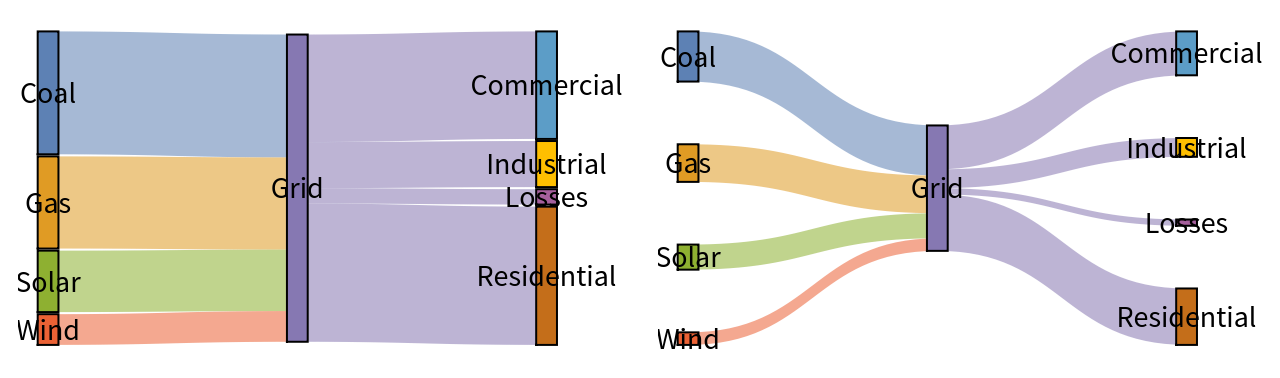
The fraction of each column's rendered height taken up by gaps between its vertices:
VertexColors (3)
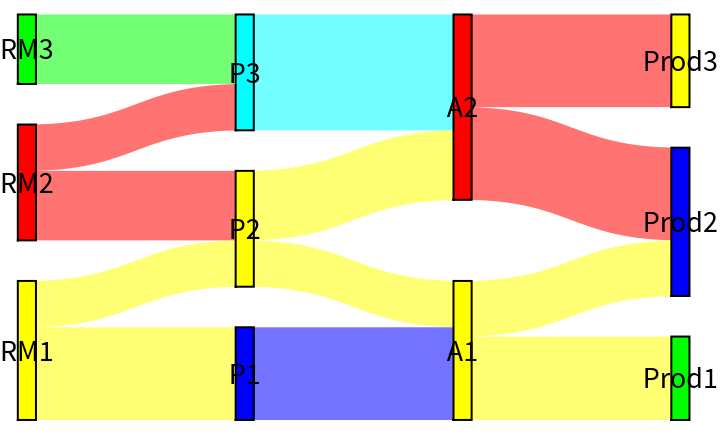
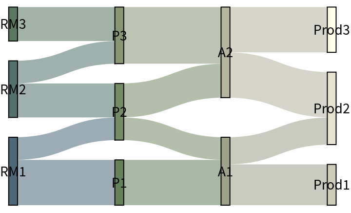
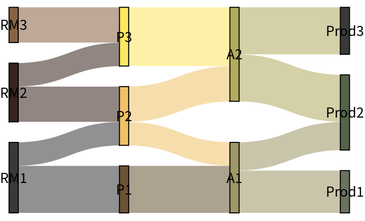
The color of vertices and the corresponding outflows are controlled by "VertexColors".
A list of colors can be provided:
A named color theme from ColorData can be used:
A numbered "Indexed" color theme can be used from ColorData:
VertexRenderingFunction (1)
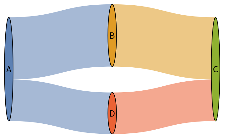
A custom Function[{centerX, centerY, width, height}, …] can draw each vertex as something other than a rectangle; the color set by "VertexColors" is prepended automatically:
EdgeOffset (1)
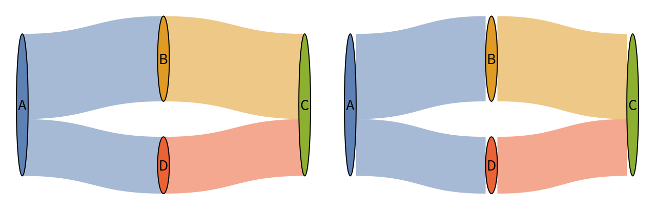
The edge flows meet behind the vertex but you can choose to space them around the vertex:
VertexLabels (2)
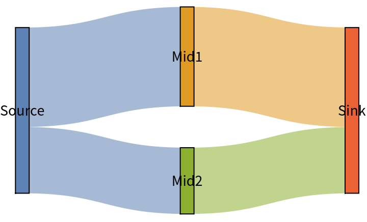
When the input is a matrix, vertices are labelled by the index number. You can override those with "VertexLabels":
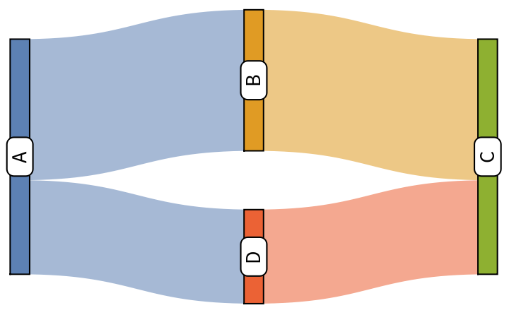
"VertexLabels" can be used to specify more complex labels that can be specified by "LabelStyle":
LayerSpacing (2)
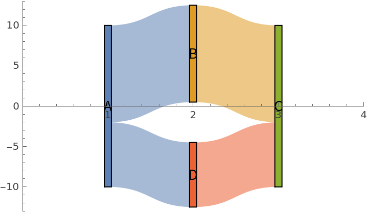
The coordinate system places vertices at integer x-positions with y-values that correspond to the flow values:
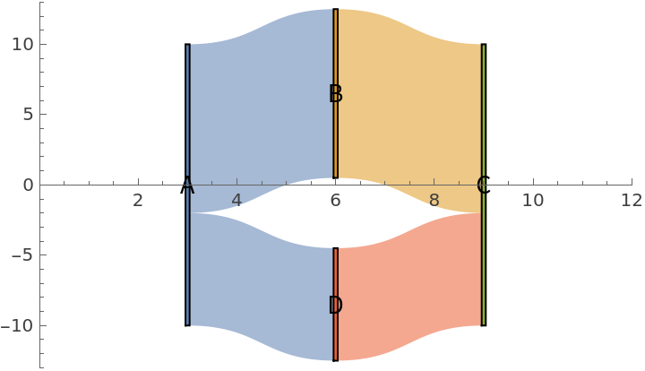
Space the vertices differently with "LayerSpacing":
VertexWidth (1)
Control the width of vertices:
OrderIterations
SankeyChart attempts to minimize the times that flows cross over each other. In complex graphs this can take time. "OrderIterations" limits the computation. The default is 8 iterations but any integer value can be used.
EdgeOpacity (1)
Outflow edges are colored the same as their source vertex but are distinguished by Opacity:
LabelStyle (1)
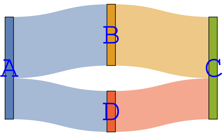
Control the appearance of text labels:
VertexPositions (2)
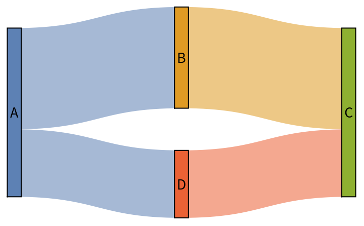
Vertices are placed automatically:
But one or more can be placed manually:
Possible Issues (1)
Vertices with only outflow are treated as sources, vertices with only inflow are treated as destinations. All other vertices must have balanced inflow and outflow must match. For example this graph has an inflow of 5 and an outflow of 10 on vertex 2:
![ResourceFunction["SankeyChart"][
Graph[{"A", "B", "C", "D"}, {"A" \[DirectedEdge] "B", "B" \[DirectedEdge] "C", "A" \[DirectedEdge] "D", "D" \[DirectedEdge] "C"}, EdgeWeight -> {12, 12, 8, 8}]]](https://www.wolframcloud.com/obj/resourcesystem/images/278/278eccb2-43e0-4d29-8899-13376e5507c2/1c917ba7d2cd7838.png)
![g2 = Graph[{"Coal", "Gas", "Solar", "Wind", "Grid", "Residential", "Commercial", "Industrial", "Losses"}, {"Coal" \[DirectedEdge] "Grid", "Gas" \[DirectedEdge] "Grid", "Solar" \[DirectedEdge] "Grid", "Wind" \[DirectedEdge] "Grid", "Grid" \[DirectedEdge] "Residential", "Grid" \[DirectedEdge] "Commercial", "Grid" \[DirectedEdge] "Industrial", "Grid" \[DirectedEdge] "Losses"}, EdgeWeight -> {40, 30, 20, 10, 45, 35, 15, 5}];
ResourceFunction["SankeyChart"][g2]](https://www.wolframcloud.com/obj/resourcesystem/images/278/278eccb2-43e0-4d29-8899-13376e5507c2/06ca45c6f4386d7f.png)
![g3 = Graph[{"RM1", "RM2", "RM3", "P1", "P2", "P3", "A1", "A2", "Prod1", "Prod2", "Prod3"}, {"RM1" \[DirectedEdge] "P1", "RM1" \[DirectedEdge] "P2", "RM2" \[DirectedEdge] "P2", "RM2" \[DirectedEdge] "P3", "RM3" \[DirectedEdge] "P3", "P1" \[DirectedEdge] "A1", DirectedEdge["P2", "A1"], "P2" \[DirectedEdge] "A2", "P3" \[DirectedEdge] "A2", "A1" \[DirectedEdge] "Prod1", "A1" \[DirectedEdge] "Prod2", "A2" \[DirectedEdge] "Prod2", "A2" \[DirectedEdge] "Prod3"}, EdgeWeight -> {20, 10, 15, 10, 15, 20, 10, 15, 25, 18, 12, 20, 20}];
ResourceFunction["SankeyChart"][g3]](https://www.wolframcloud.com/obj/resourcesystem/images/278/278eccb2-43e0-4d29-8899-13376e5507c2/4ee3fad7af3e1c99.png)
![matrix = {{0, 12, 8, 0}, {0, 0, 0, 12}, {0, 0, 0, 8}, {0, 0, 0, 0}};
ResourceFunction["SankeyChart"][matrix, "VertexLabels" -> {"A", "B", "C", "D"}]](https://www.wolframcloud.com/obj/resourcesystem/images/278/278eccb2-43e0-4d29-8899-13376e5507c2/78c949ba46300434.png)
![flowGraph = \!\(\*
GraphicsBox[
NamespaceBox["NetworkGraphics",
DynamicModuleBox[{Typeset`graph = HoldComplete[
Graph[{1, 2, 3, 4}, {{{1, 2}, {1, 3}, {2, 4}, {3, 4}}, Null}, {EdgeCapacity -> {10, 5, 10, 5}}]]},
TagBox[GraphicsGroupBox[
GraphicsComplexBox[{{-1.8369701987210297`*^-16, 1.}, {1., 1.2246467991473532`*^-16}, {-1., -2.4492935982947064`*^-16}, {6.123233995736766*^-17, -1.}}, {
{Hue[0.6, 0.7, 0.7], Opacity[0.7], CapForm["Round"], Arrowheads[
Medium], ArrowBox[{{1, 2}, {1, 3}, {2, 4}, {3, 4}}, 0.02261146496815286]},
{Hue[0.6, 0.5, 1.], EdgeForm[{GrayLevel[0], Opacity[0.7]}], DiskBox[1, 0.02261146496815286], DiskBox[2, 0.02261146496815286], DiskBox[3, 0.02261146496815286], DiskBox[4, 0.02261146496815286]}}]],
MouseAppearanceTag["NetworkGraphics"]],
AllowKernelInitialization->False]],
DefaultBaseStyle->"NetworkGraphics",
FormatType->TraditionalForm,
FrameTicks->None,
ImageSize->{74.359375, Automatic}]\);
flowData = FindMaximumFlow[flowGraph, 1, 4, "OptimumFlowData"];
ResourceFunction["SankeyChart"][flowData]](https://www.wolframcloud.com/obj/resourcesystem/images/278/278eccb2-43e0-4d29-8899-13376e5507c2/6d910021ef481820.png)
![ResourceFunction["SankeyChart"][
Graph[{"S", "A", "B", "D", "F"}, {"S" \[DirectedEdge] "A", "D" \[DirectedEdge] "A", "A" \[DirectedEdge] "B", "D" \[DirectedEdge] "B", "B" \[DirectedEdge] "D", "D" \[DirectedEdge] "F"}, EdgeWeight -> {10, 3, 13, 2, 15, 10}]]](https://www.wolframcloud.com/obj/resourcesystem/images/278/278eccb2-43e0-4d29-8899-13376e5507c2/39bf39e3775be01d.png)
![g2 = Graph[{"Coal", "Gas", "Solar", "Wind", "Grid", "Residential", "Commercial", "Industrial", "Losses"}, {"Coal" \[DirectedEdge] "Grid", "Gas" \[DirectedEdge] "Grid", "Solar" \[DirectedEdge] "Grid", "Wind" \[DirectedEdge] "Grid", "Grid" \[DirectedEdge] "Residential", "Grid" \[DirectedEdge] "Commercial", "Grid" \[DirectedEdge] "Industrial", "Grid" \[DirectedEdge] "Losses"}, EdgeWeight -> {40, 30, 20, 10, 45, 35, 15, 5}]; ResourceFunction[
"SankeyChart"][g2, "EdgeOrigin" -> Top]](https://www.wolframcloud.com/obj/resourcesystem/images/278/278eccb2-43e0-4d29-8899-13376e5507c2/3da07722bbd0a6a6.png)
![g = Graph[{"A", "B", "C", "D"}, {"A" \[DirectedEdge] "B", "B" \[DirectedEdge] "C", "A" \[DirectedEdge] "D", "D" \[DirectedEdge] "C"}, EdgeWeight -> {12, 12, 8, 8}];
ResourceFunction["SankeyChart"][g, "VertexLabelPosition" -> #, PlotLabel -> #] & /@ {Center, None, Above, Below, Top, Bottom, 1, -1, 0}](https://www.wolframcloud.com/obj/resourcesystem/images/278/278eccb2-43e0-4d29-8899-13376e5507c2/702d6e790274456c.png)
![ResourceFunction["SankeyChart"][g, "VertexLabelPosition" -> {Center, #}, PlotLabel -> {Center, #}] & /@ {Left, Right, Center, 5, -5}](https://www.wolframcloud.com/obj/resourcesystem/images/278/278eccb2-43e0-4d29-8899-13376e5507c2/773c6dacd686e4a6.png)
![g = Graph[{"A", "B", "C", "D"}, {"A" \[DirectedEdge] "B", "B" \[DirectedEdge] "C", "A" \[DirectedEdge] "D", "D" \[DirectedEdge] "C"}, EdgeWeight -> {12, 12, 8, 8}];
ResourceFunction["SankeyChart"][g, "VertexLabelPosition" -> Top, "VertexValuePosition" -> Bottom]](https://www.wolframcloud.com/obj/resourcesystem/images/278/278eccb2-43e0-4d29-8899-13376e5507c2/7978d26139156cb1.png)
![g2 = Graph[{"Coal", "Gas", "Solar", "Wind", "Grid", "Residential", "Commercial", "Industrial", "Losses"}, {"Coal" \[DirectedEdge] "Grid", "Gas" \[DirectedEdge] "Grid", "Solar" \[DirectedEdge] "Grid", "Wind" \[DirectedEdge] "Grid", "Grid" \[DirectedEdge] "Residential", "Grid" \[DirectedEdge] "Commercial", "Grid" \[DirectedEdge] "Industrial", "Grid" \[DirectedEdge] "Losses"}, EdgeWeight -> {40, 30, 20, 10, 45, 35, 15, 5}];
ResourceFunction["SankeyChart"][g2, "EdgeValuePosition" -> Center]](https://www.wolframcloud.com/obj/resourcesystem/images/278/278eccb2-43e0-4d29-8899-13376e5507c2/30821ae6e8a6aac0.png)
![g2 = Graph[{"Coal", "Gas", "Solar", "Wind", "Grid", "Residential", "Commercial", "Industrial", "Losses"}, {"Coal" \[DirectedEdge] "Grid", "Gas" \[DirectedEdge] "Grid", "Solar" \[DirectedEdge] "Grid", "Wind" \[DirectedEdge] "Grid", "Grid" \[DirectedEdge] "Residential", "Grid" \[DirectedEdge] "Commercial", "Grid" \[DirectedEdge] "Industrial", "Grid" \[DirectedEdge] "Losses"}, EdgeWeight -> {40, 30, 20, 10, 45, 35, 15, 5}];
GraphicsRow[{ResourceFunction["SankeyChart"][g2, "VertexSpacing" -> 0.02], ResourceFunction["SankeyChart"][g2, "VertexSpacing" -> 0.6]}]](https://www.wolframcloud.com/obj/resourcesystem/images/278/278eccb2-43e0-4d29-8899-13376e5507c2/177c5816f6e75fdf.png)
![g3 = Graph[{"RM1", "RM2", "RM3", "P1", "P2", "P3", "A1", "A2", "Prod1", "Prod2", "Prod3"}, {"RM1" \[DirectedEdge] "P1", "RM1" \[DirectedEdge] "P2", "RM2" \[DirectedEdge] "P2", "RM2" \[DirectedEdge] "P3", "RM3" \[DirectedEdge] "P3", "P1" \[DirectedEdge] "A1", DirectedEdge["P2", "A1"], "P2" \[DirectedEdge] "A2", "P3" \[DirectedEdge] "A2", "A1" \[DirectedEdge] "Prod1", "A1" \[DirectedEdge] "Prod2", "A2" \[DirectedEdge] "Prod2", "A2" \[DirectedEdge] "Prod3"}, EdgeWeight -> {20, 10, 15, 10, 15, 20, 10, 15, 25, 18, 12, 20, 20}];
ResourceFunction["SankeyChart"][g3, "VertexColors" -> {Yellow, Red, Green, Blue, Yellow, Cyan}]](https://www.wolframcloud.com/obj/resourcesystem/images/278/278eccb2-43e0-4d29-8899-13376e5507c2/24b3193551c2d0ec.png)
![ResourceFunction["SankeyChart"][g3, "VertexColors" -> "AlpineColors"]](https://www.wolframcloud.com/obj/resourcesystem/images/278/278eccb2-43e0-4d29-8899-13376e5507c2/5f20ea8b4468772f.png)
![ResourceFunction["SankeyChart"][g3, "VertexColors" -> 4]](https://www.wolframcloud.com/obj/resourcesystem/images/278/278eccb2-43e0-4d29-8899-13376e5507c2/70f5cda9269575d6.png)
![g = Graph[{"A", "B", "C", "D"}, {"A" \[DirectedEdge] "B", "B" \[DirectedEdge] "C", "A" \[DirectedEdge] "D", "D" \[DirectedEdge] "C"}, EdgeWeight -> {12, 12, 8, 8}]; ResourceFunction["SankeyChart"][g, "VertexRenderingFunction" -> Function[{x, y, w, h}, {EdgeForm[Black], Disk[{x, y}, {w/2, h/2}]}]]](https://www.wolframcloud.com/obj/resourcesystem/images/278/278eccb2-43e0-4d29-8899-13376e5507c2/2373bb31bd95dbf0.png)
![g=Graph[{"A","B","C","D"},{"A"\[DirectedEdge]"B","B"\[DirectedEdge]"C","A"\[DirectedEdge]"D","D"\[DirectedEdge]"C"},EdgeWeight->{12,12,8,8}];
diskFn = Function[{x, y, w, h}, {EdgeForm[Black], Disk[{x, y}, {w/2, h/2}]}];
GraphicsRow[{SankeyChart[g, "VertexRenderingFunction" -> diskFn, "EdgeOffset" -> 0],
SankeyChart[g, "VertexRenderingFunction" -> diskFn, "EdgeOffset" -> 1]
}]](https://www.wolframcloud.com/obj/resourcesystem/images/278/278eccb2-43e0-4d29-8899-13376e5507c2/7a05b5e4c1930277.png)
![matrix = {{0, 12, 8, 0}, {0, 0, 0, 12}, {0, 0, 0, 8}, {0, 0, 0, 0}};
ResourceFunction["SankeyChart"][matrix, "VertexLabels" -> {"Source", "Mid1", "Mid2", "Sink"}]](https://www.wolframcloud.com/obj/resourcesystem/images/278/278eccb2-43e0-4d29-8899-13376e5507c2/5d54c150bff16287.png)
![g = Graph[{"A", "B", "C", "D"}, {"A" \[DirectedEdge] "B", "B" \[DirectedEdge] "C", "A" \[DirectedEdge] "D", "D" \[DirectedEdge] "C"}, EdgeWeight -> {12, 12, 8, 8}];
ResourceFunction["SankeyChart"][g,
"VertexLabels" -> (Framed[Rotate[#, Pi/2], Background -> White, RoundingRadius -> 5] & /@ {"A", "B", "C", "D"})
]](https://www.wolframcloud.com/obj/resourcesystem/images/278/278eccb2-43e0-4d29-8899-13376e5507c2/40e629064a0f709a.png)
![g = Graph[{"A", "B", "C", "D"}, {"A" \[DirectedEdge] "B", "B" \[DirectedEdge] "C", "A" \[DirectedEdge] "D", "D" \[DirectedEdge] "C"}, EdgeWeight -> {12, 12, 8, 8}];
ResourceFunction["SankeyChart"][g, Axes -> True, PlotRange -> {{0, 4}, Automatic}]](https://www.wolframcloud.com/obj/resourcesystem/images/278/278eccb2-43e0-4d29-8899-13376e5507c2/2add82a200fa4e10.png)
![g = Graph[{"A", "B", "C", "D"}, {"A" \[DirectedEdge] "B", "B" \[DirectedEdge] "C", "A" \[DirectedEdge] "D", "D" \[DirectedEdge] "C"}, EdgeWeight -> {12, 12, 8, 8}];
ResourceFunction["SankeyChart"][g, Axes -> True, PlotRange -> {{0, 12}, Automatic}, "LayerSpacing" -> 3]](https://www.wolframcloud.com/obj/resourcesystem/images/278/278eccb2-43e0-4d29-8899-13376e5507c2/75ae287e9546a3ad.png)
![g = Graph[{"A", "B", "C", "D"}, {"A" \[DirectedEdge] "B", "B" \[DirectedEdge] "C", "A" \[DirectedEdge] "D", "D" \[DirectedEdge] "C"}, EdgeWeight -> {12, 12, 8, 8}];
ResourceFunction["SankeyChart"][g, "VertexWidth" -> #] & /@ {0.05, 0.2, 0.5}](https://www.wolframcloud.com/obj/resourcesystem/images/278/278eccb2-43e0-4d29-8899-13376e5507c2/251f397ab8a8c606.png)

![g = Graph[{"A", "B", "C", "D"}, {"A" \[DirectedEdge] "B", "B" \[DirectedEdge] "C", "A" \[DirectedEdge] "D", "D" \[DirectedEdge] "C"}, EdgeWeight -> {12, 12, 8, 8}];
ResourceFunction["SankeyChart"][g, "EdgeOpacity" -> #] & /@ {0.2, 0.5,
1}](https://www.wolframcloud.com/obj/resourcesystem/images/278/278eccb2-43e0-4d29-8899-13376e5507c2/095bb7f6dc4880e6.png)

![g = Graph[{"A", "B", "C", "D"}, {"A" \[DirectedEdge] "B", "B" \[DirectedEdge] "C", "A" \[DirectedEdge] "D", "D" \[DirectedEdge] "C"}, EdgeWeight -> {12, 12, 8, 8}];
ResourceFunction["SankeyChart"][g, LabelStyle -> {FontSize -> 50, FontColor -> Blue, FontFamily -> "Courier New"}]](https://www.wolframcloud.com/obj/resourcesystem/images/278/278eccb2-43e0-4d29-8899-13376e5507c2/7a3100f7d1f9d703.png)
![g = Graph[{"A", "B", "C", "D"}, {"A" \[DirectedEdge] "B", "B" \[DirectedEdge] "C", "A" \[DirectedEdge] "D", "D" \[DirectedEdge] "C"}, EdgeWeight -> {12, 12, 8, 8}];
ResourceFunction["SankeyChart"][g]](https://www.wolframcloud.com/obj/resourcesystem/images/278/278eccb2-43e0-4d29-8899-13376e5507c2/3af68947fe6438f7.png)
![g = Graph[{"A", "B", "C", "D"}, {"A" \[DirectedEdge] "B", "B" \[DirectedEdge] "C", "A" \[DirectedEdge] "D", "D" \[DirectedEdge] "C"}, EdgeWeight -> {12, 12, 8, 8}];
ResourceFunction["SankeyChart"][g, "VertexPositions" -> {"B" -> {2.5, 10}} ]](https://www.wolframcloud.com/obj/resourcesystem/images/278/278eccb2-43e0-4d29-8899-13376e5507c2/20a1ee3af358673a.png)
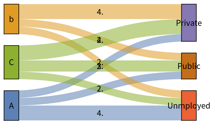
![ResourceFunction[
"AlluvialFlowChart"][{{(*A->{Public,Private,
Unemployed}*){4, 2, 2},(*B*){2, 4, 2},(*C*){2, 4, 3}}}, {(*district*){"A", "B", "C"},(*employed*){"Public", "Private", "Unemployed"}},(*stages*){"District", "Employment"}, "ImageSize" -> 400]](https://www.wolframcloud.com/obj/resourcesystem/images/278/278eccb2-43e0-4d29-8899-13376e5507c2/567ced0f536e31a9.png)

![ResourceFunction["SankeyChart"][WeightedAdjacencyGraph[
{(*A->{Public,Private,Unemployed}*)
{0, 0, 0, 4, 2, 2},
(*B*){0, 0, 0, 2, 4, 2},
(*C*){0, 0, 0, 2, 4, 3}, {4, 2, 2, 0, 0, 0},
{2, 4, 4, 0, 0, 0},
(*C*){2, 2, 3, 0, 0, 0} }], "VertexLabels" -> {"A", "b", "C", "Unmployed", "Private", "Public"}, "EdgeValuePosition" -> Center]](https://www.wolframcloud.com/obj/resourcesystem/images/278/278eccb2-43e0-4d29-8899-13376e5507c2/515da868663a7f90.png)
![badGraph = Graph[{1, 2, 3}, {1 \[DirectedEdge] 2, 2 \[DirectedEdge] 3}, EdgeWeight -> {5, 10}];
ResourceFunction["SankeyChart"][badGraph]](https://www.wolframcloud.com/obj/resourcesystem/images/278/278eccb2-43e0-4d29-8899-13376e5507c2/65ff1e4c585f4832.png)

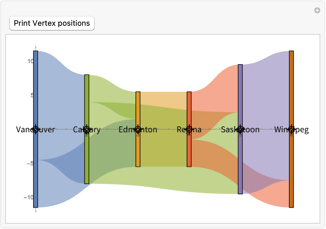
![Manipulate[
ResourceFunction[
"SankeyChart"][{{0, 7, 16, 0, 0, 0}, {0, 0, 0, 11, 0, 0}, {0, 4, 0, 0, 12, 0}, {0, 0, 0, 0, 7, 4}, {0, 0, 0, 0, 0, 19}, {0, 0, 0, 0, 0, 0}},
"VertexLabels" -> {"Vancouver", "Edmonton", "Calgary", "Regina", "Saskatoon", "Winnipeg"}, Axes -> True,
"VertexPositions" -> MapThread[
Rule, {{"Vancouver", "Calgary", "Edmonton", "Regina", "Saskatoon",
"Winnipeg"}, loc}], ImageSize -> 500],
{{loc, {#, 0} & /@ Range[6]}, Locator},
Button["Print Vertex positions", Print["VertexPositions" -> MapThread[
Rule, {{"Vancouver", "Calgary", "Edmonton", "Regina", "Saskatoon",
"Winnipeg"}, loc}]]]]](https://www.wolframcloud.com/obj/resourcesystem/images/278/278eccb2-43e0-4d29-8899-13376e5507c2/3d17c53b23b14cdf.png)